University of Warwick institutional repository: http://go.warwick.ac.uk/wrap
This paper is made available online in accordance with
publisher policies. Please scroll down to view the document
itself. Please refer to the repository record for this item and our
policy information available from the repository home page for
further information.
To see the final version of this paper please visit the publisher’s website
.
Access to the published version may require a subscription.
Author(s): CFH Nam, JAD Aston and AM Johansen
Article Title: Quantifying the Uncertainty in Change Points
Year of publication: 2011
Link to published article:
http://www2.warwick.ac.uk/fac/sci/statistics/crism/research/2011/paper
11-19/
Quantifying the Uncertainty in Change Points
Christopher F. H. Nam, John A. D. Aston and Adam M. Johansen,
Department of Statistics, University of Warwick, Coventry, CV4 7AL, UK
{
c.f.h.nam
|
j.a.d.aston
|
a.m.johansen
}
@warwick.ac.uk
May 31, 2011
Abstract
Quantifying the uncertainty in the location and nature of change points in time series is important
in a variety of applications. Many existing methods for estimation of the number and location of
change points fail to capture fully or explicitly the uncertainty regarding these estimates, whilst
others require explicit simulation of large vectors of dependent latent variables.
This paper proposes methodology for approximating the full posterior distribution of various
change point characteristics in the presence of parameter uncertainty. The methodology combines
recent work on evaluation of exact change point distributions conditional on model parameters via
Finite Markov Chain Imbedding in a Hidden Markov Model setting, and accounting for parameter
uncertainty and estimation via Bayesian modelling and Sequential Monte Carlo. The combination of
the two leads to a flexible and computationally efficient procedure, which does not require estimates
of the underlying state sequence.
We illustrate that good estimation of posterior distributions regarding change point characteristics
is provided for simulated and functional magnetic resonance imaging data. We use the methodology
to show that the modelling of relevant physical properties of the scanner can influence detection of
change points and their uncertainty.
Keywords: Change Points; Finite Markov Chain Imbedding; Functional Magnetic Resonance Imaging; Hidden Markov Models; Sequential Monte Carlo; Segmentation
1
Introduction
Detecting and estimating the number and location of change points in time series is becoming
increas-ingly important as both a theoretical research problem and a necessary part of applied data analysis.
Originating in the 1950s in a quality control setting (Page, 1954), there are numerous existing approaches,
both parametric and non-parametric, often requiring strong assumptions upon the type of changes that
can occur and the distribution of the data. We refer the reader to Chen and Gupta (2000); Eckley et al.
problems appear under various names including segmentation, novelty detection, structural break
identi-fication, and disorder detection. These approaches however, typically fail to fully capture uncertainty in
the number and location of these change points. For example, model selection and optimal segmentation
based techniques (for example Yao (1988); Davis et al. (2006)) rely on asymptotic arguments on
pro-viding consistent estimates of the number of change points present, whilst others assume the number of
change points to be known, in order to consider the uncertainty regarding the locations of these change
points (see Chib (1998); Stephens (1994)). Those methods which do fully characterise the uncertainty
involved typically require simulation of large vectors of correlated latent variables. This paper proposes a
methodology which fully quantifies the uncertainty of change points for an observed time series, without
estimating or simulating the unobserved state sequence.
Our proposed methodology is based upon three areas of existing work. We model our observed time
series and consider change points in a Hidden Markov Model (HMM) framework. HMMs and the general
use of dependent latent state variables are widely used in change point estimation (Chib, 1998; Fearnhead,
2006; Fearnhead and Liu, 2007). In these approaches, each state of the underlying chain represents a
segment of data between change points and thus a change point is said to occur when there is a change
in state in the underlying chain. The underlying chain is constructed so that there are only two possible
moves; either stay in the same state (no change point has occurred), or move to the next state in the
sequence, corresponding to a new segment and thus a change point has occurred. Interest now lies
predominantly in determining the latent state sequence (usually through simulation, by Markov Chain
Monte Carlo (MCMC) for example), in order to determine the relevant change point characteristics. We
note that under the framework of Chib (1998), the number of change points is assumed to be known
since this is related to the number of states of the imposed HMM. However, this is quite restrictive and
makes sense only in those settings in which return to a previously visited segment and state is regarded
as impossible.
We consider an alternative approach by using HMMs in their usual context, where each state
rep-resents different data generating mechanisms (for example the “good” and “bad” states when using a
Poisson HMM to model the number of daily epileptic seizure counts Albert (1991)) and returning to
previously visited states is possible. This allows the number of change points to be unknown a priori and
inferred from the data. We do at present assume that the number of different states is known although
the method can be extended to the more general case. This latter point seems less restrictive in a change
point context than assuming the number of change points to be known given the quantities of interest.
We also consider a generalised definition of change points corresponding to asustainedchange in the
underlying state sequence. This means that we are looking for runs of particular states in the underlying
state sequence: determining that a change point to a particular regime has occurred when a particular
sequence of states is observed. We employ Finite Markov Chain Imbedding (FMCI) (Fu and Koutras,
1994; Fu and Lou, 2003), an elegant framework which allows distributions regarding run and pattern
error.
The above techniques allow exact change point distributions to be computed. However, these
dis-tributions are conditional upon the model parameters. In practice, it is common for these parameters
to be treated as known, with maximum likelihood estimates being used. However, in most applications
where parameters are estimated from the data itself, it is desirable to account for parameter uncertainty
in change point estimates. If a Bayesian approach to the characterisation of changes is employed, then it
would also seem desirable to take a Bayesian approach to the characterisation of parameter uncertainty.
Recent Bayesian change point approaches have dealt with model parameter uncertainty by integrating
the parameters out in some fashion in order to ultimately sample from the joint posterior of the location
and number of change points, usually achieved by also sampling the aforementioned latent state sequence
(Fearnhead, 2006; Chib, 1998). However, this introduces additional sampling error into the change point
estimates and requires the simulation of the underlying state sequence which is often long and highly
correlated — and thus hard to sample efficiently. We consider model parameter uncertainty by sampling
from the the posterior distribution of the model parameters via Sequential Monte Carlo, without
simu-lating the latent state sequences. This approach introduces sampling error only in the model parameters
and retains, conditionally, the exact change point distributions: we will show that this amounts to a
Rao-Blackwellized form of the estimator.
Quantifying the uncertainty in change point problems is often overlooked but nevertheless an
impor-tant aspect of inference. Whilst, quite naturally, more emphasis has typically been placed on detection
and estimation in problems, quantifying the uncertainty of change points can lead to a better
under-standing of the data and the system generating the data. Whenever estimates are provided for the
location of change points, we should be interested in determining how confident we can be about these
estimates, and whether other change point configurations are plausible. In many situations it may be
desirable to average over models rather than choosing a most probable explanation. Alternatively, we
may want to assess the confidence we have in the estimate of the number of change points and if there is
any substantial probability of any other number of change points having occurred. In addition, different
change point approaches can often lead to different estimates when applied to the same time series; this
motivates the assessment of the performance and plausibility of these different approaches and their
estimates. Quantifying the uncertainty provides a means of so doing.
The exact change point distributions computed via FMCI methodology (Aston et al., 2009) already
quantify the residual uncertainty given both the model parameters and the observed data. However,
this conditioning on the model parameters is typically difficult to justify. It is important to consider
also parameter uncertainty because the use of different model parameters can give quite different change
point results and thus conclusions. This effect becomes more important when there are several different
competing model parameter values which provide equally-plausible explanations of the data. By
con-sidering model parameter uncertainty within the quantification of uncertainty for change points, we are
thus fully quantifies the uncertainty regarding change points. This will be seen to be especially true in
the analysis of functional Magnetic Resonance Imaging (fMRI) time series.
When analysing fMRI data, it is common to assume that the data arises from a known experimental
design (Worsley et al., 2002). However, this assumption is very restrictive particularly in experiments
common in psychology where the exact timing of the expected reaction is unknown, with different
subjects reacting at different times and in different ways to an equivalent stimulus (Lindquist et al.,
2007). Change point methodology has therefore been proposed as a possible solution to this problem,
where the change points effectively act as a latent design for each time series. Significant work has been
done in designing methodology for these situations for the at-most-one-change situation using control
chart type methods (Lindquist et al., 2007; Robinson et al., 2010). Using the methodology developed in
this paper, we are able to define an alternative approach based on HMMs that allows not only multiple
change points to be taken into account, but also the inclusion of an autoregressive (AR) error process
assumptions and detrending within a unified analysis. These features need to be accounted for in fMRI
time series (Worsley et al., 2002) and will be shown to have an effect on the conclusions that can be
drawn from the associated analysis.
The remainder of this paper has the following structure: Section 2 details the statistical background
of the methodology which is proposed in Section 3. This methodology is applied to both simulated and
fMRI data in Section 4. We conclude in Section 5 with some discussion of our findings.
2
Background
Lety1, y2, . . . , yn be an observed non-stationary time series with respect to a varying second order
struc-ture. One particular framework for modelling such a time series is via Hidden Markov Models (HMMs)
where the observation process {Yt}t>0 is conditionally independent given an unobserved underlying
Markov chain{Xt}t>0. The states of the underlying chain correspond to different data generating
mech-anisms, with each state characterised by a collection of parameter values. The methods presented in this
paper can be applied to general finite state Hidden Markov Models (including Markov switching models)
with finite dependency on previous states of the underlying chain. This class of HMMs are of the form:
yt|y1:t−1, x1:t∼f(yt|xt−r:t, y1:t−1, θ) (Emission) (1)
p(xt|x1:t−1, y1:t−1, θ) =p(xt|xt−1, θ) t= 1, . . . , n (Transition).
Given the set of model parameters θ, the observation at time t = 1, . . . , n, yt has emission density
de-pendent of previous observations y1:t−1 and previous r states of the underlying states xt−r, . . . , xt−1.
We use the common shorthand notation of yt1:t2 = (yt1, yt1+1, . . . , yt2) and analogously forxt1:t2. The
underlying states are assumed to follow a first order Markov chain (although standard embedding
ar-guments would in principle allow generalisation to anmth order Markov chain) and takes values in the
model but typically consist of transition probabilities for the underlying Markov chain, and parameters
relating to the emission density. For good overviews of HMMs, we refer the reader to MacDonald and
Zucchini (1997); Capp´e et al. (2005).
A common definition within an HMM framework is that a change point has occurred at time t
whenever there is a change in the underlying chain, that is xt−1 6= xt. This definition is currently
adopted in existing works such as Chib (1998); Hamilton (1989); Durbin et al. (1998); Fearnhead (2006).
However, we consider a slightly more general definition; a change point to a regime occurs at timetwhen
the change in the underlying chain persists for at leastk time periods. That isxt−16=xt=. . .=xt+j
where j ≥ k−1, and the term “regime” refers more specifically to observations from the sustained
movement in the underlying chain. Although this definition can be interpreted as an instance of the
simpler definition defined on a suitably expanded space, it is both easier to interpret and computationally
convenient to make use of this explicit form. The motivation for this generalised definition is that there
are several applications and scenarios in which a sustained change is required before a change to a new
regime is said to have occurred. Typical examples include Economics where a recession is said to have
occurred when there are at least two consecutive negative growth (contraction) states and thusk= 2, or
in Genetics where a specific genetic phenomena, for example a CpG island (Aston and Martin, 2007), is
at least a few hundred bases long (for examplek= 1000) before being deemed in progress. The standard
change point definition can be recovered by settingk= 1.
Interest often lies in determining the time of a change point and the number of change points occurring
within a time series. Let M(k)and τ(k)= (τ1(k), . . . , τM(k)(k)) be variables denoting the number and times
of change points, respectively. Given a vectorτ(k) we uset ∈τ(k) to indicate that one of the elements of τ(k) is equal to t: if t ∈τ(k), then∃j ∈ {1, . . . , M(k)} such that τ(k)
j =t. The goal of this paper is
quantifying the uncertainty of these characteristics by estimating:
P(M(k)=m|y1:n) m= 0,1,2,3, . . . , (2)
andP
τ(k)3t|y1:n
(3)
where P(τ(k)3t|y 1:n) =
P
mP(M
(k)=m|y 1:n)
Pm
i=1P(τ
(k)
i =t|y1:n, M(k)=m). That is, the
proba-bility distribution of the number of changes and the marginal posterior probaproba-bility that a change point
occurs at any particular time.
2.1
Exact Change Point Distributions using Finite Markov Chain Imbedding
Under this generalised change point setting and conditioned on a particular model parameter settingθ,
it is possible to compute exact distributions regarding change point characteristics (Aston et al., 2009).
That is, it is possible to computeP(τ(k)3t|y
1:n, θ) andP(M(k)=m|y1:n, θ) exactly, where exact means
that they are not subject to sampling or approximation error.
The generalised definition of a change point consequently motivates that we are looking for runs of
occurrences of s. That is,xt =s=xt+1 =. . . =xt+k−1, and in this instance, if xt−1 6=s the run of
desired lengthk has occurred at timet+k−1. Thus in order to consider whether a change point has
occurred by time t, we can reformulate this problem to whether a run of length exactlyk has occurred
at timet+k−1 in the underlying chain.
One popular approach for analysing behaviour in the underlying state sequence for HMMs is to
pro-vide an estimate of the underlying state sequence using techniques such as the Viterbi algorithm (Viterbi,
1967) and posterior decoding (Baum et al., 1970). These provide the most probable state sequence and
the sequence which maximises a marginal probability of the states at each time respectively. Subsequent
inference is often performed conditioned upon these point estimates which are subsequently assumed to
be known — all runs and pattern statistics are derived conditional upon the estimated parameter values
and the given sequence. This approach fails to capture the uncertainty arising from the unknown latent
state sequence and thus for the run and pattern statistics of interest (as all inference is based on this
single state sequence estimate), leading to a systematic underestimation of the attendant uncertainty.
In addition, posterior decoding can produce estimates which feature impossible state transitions due
to its reliance upon marginal distributions. We consider an alternative approach: in order to quantify
fully the uncertainty of change points it is necessary to consider all possible state sequences. This is
achieved by computing time-inhomogeneous transition probabilities with respect to the observed time
series, p(xt|xt−1, y1:n),∀t = 1, . . . , n, which can be obtained from smoothing probabilities. This thus
allows us to quantify the uncertainty regarding runs in the underlying Markov chain and ultimately the
change points themselves.
Let τu(k) denote the time of the uth change point with u≥1. We can decompose the change point
probability of interest into:
P(τ(k)3t|y1:n, θ) =
X
m
P(M(k)=m)
m
X
u=1
P(τu(k)=t|M(k)=m, y1:n) (4)
= X
u=1,2,...
P(τu(k)=t, M(k)≥u|y1:n, θ). (5)
The event of theuth change point occurring at timet can be re-expressed as a quantity involving runs,
namely whether theuth run of minimum lengthkhas occurred at timet+k−1. LetWs(k, u) denote the
waiting time for the uth occurrence of a run of minimum length k in states∈ΩX. ThusWs(k, u) =t
denotes that at timet, theuth occurrence of a such a run occurs. W(k, u) similarly denotes the waiting
time for the uth occurrence of a run in any state s∈ΩX of at least length k. If change points into a
certain regime were of interest,Ws(k, u) wheres∈ΩX is the state defining the regime of interest, is of
greater interest. By re-expressing theuth change point event as the waiting time for theuth occurrence
of a run, it is thus possible to compute the corresponding probabilities:
P(τu(k)=t|y1:n, θ) =P(W(k, u) =t+k−1|y1:n, θ). (6)
It is possible to compute exactly the distribution of waiting time statistics, namely P(W(k, u) ≤
FMCI introduces several auxiliary Markov processes, {Zt(1), Zt(2), Zt(3), . . .} which are defined over the common state space Ω(Zk)= ΩX× {−1,0,1, . . . , k}. Ω
(k)
Z is an expanded version of ΩX which consists of
tuples (Xt, j) where the new variable j =−1,0,1,2. . . , k indicates the progress of any potential runs.
The auxiliary processes are constructed such that theuth process corresponds to the conditional Markov
chain for finding a run of length k, conditional on the fact that u−1 runs of length at least k have
already occurred multiplied by the conditional probability ofu−1 runs having occurred.
The states of the auxiliary Markov chains can loosely be categorised into three categories:
continua-tion (j=−1), run in progress (j= 0,1,2, . . . , k−1) and absorption (j=k). Absorption states denote
that the run of required length has occurred, the run in progress states are fairly self explanatory, and
continuation states denote when the (u−1)th run is still in progress (its length exceeds the required
length ofk) and needs to end before the occurrence of the newuth run can be considered. The transition
probabilities of these auxiliary Markov chains {Zt(1), Zt(2), Zt(3), . . .} are obtained deterministically from those of the original Markov chain {Xt}. In an HMM framework, the time-inhomogeneous posterior
transition probabilities are used in order to account for all possible state sequences given the observed
time series.
Thus in order to determine whether the specific occurrence of a run has occurred by a specific time,
we simply need to determine if the corresponding auxiliary Markov chain has reached the absorption
set,A, the set of all absorption states, by the specified time. The corresponding probability can thus be
computed by standard Markov chain results. This leads to computing the probability of theuth change
point probability.
P(W(k, u)≤t+k−1|y1:n, θ) =P(Z
(u)
t+k−1∈A|y1:n, θ) (7)
P(τu(k)=t|y1:n, θ) =P(W(k, u) =t+k−1|y1:n, θ) (8)
=P(W(k, u)≤t+k−1|y1:n, θ)−P(W(k, u)≤t+k−2|y1:n, θ). (9)
The distribution of the number of change points can also be computed from these waiting time
distribu-tions:
P(M(k)=m|y1:n, θ) =P(W(k, u)≤n|y1:n, θ)−P(W(k, u+ 1)≤n|y1:n, θ) (10)
In general, this FMCI approach allows for exact computation of distributions for other change point
characteristics such as the probability of a change within a given time interval and the distribution of
the regime durations. This thus provides a flexible methodology in capturing the uncertainty of change
point problems.
However, these distributions of change point characteristics are conditioned on the model parameters
θ. However, it is typical forθto be unknown, and subject to error and uncertainty (for example estimation
error). Thus, in order fully consider uncertainty in change points, it is necessary to also consider the
uncertainty of the parameters. We can account for model parameters via the use of Sequential Monte
2.2
Sequential Monte Carlo samplers
In order to deal with parameter uncertainty, we adopt a Bayesian approach by integrating out the model
parameters to obtain a marginal posterior distribution on the change point quantities alone. However,
it is not feasible to perform this integration analytically for the models of interest.
Sequential Monte Carlo (SMC) methods are a class of simulation algorithms for sampling from a
sequence of related distributions,{πb}Bb=1, via importance sampling and resampling techniques. Common
applications of these methods in Statistics, Engineering and related disciplines include sampling from a
sequence of posteriors as data becomes available and the particle filter for approximating the optimal
filter (to obtain the distribution of the underlying state sequence as observations become available) in
general (typically continuous) state space nonlinear and non-Gaussian HMMs (Gordon et al., 1993); see
Doucet and Johansen (2011) for a recent survey. We do not use SMC to infer on the underlying state
sequence in our particular context because the state sequence is ultimately of little interest to us and we
can calculate quantities of interest marginally.
The standard application of SMC techniques requires that the sequence of distributions of interest are
defined upon a sequence of increasing state spaces and that one is interested in only particular marginal
distributions. Sequential Monte Carlo samplers (Del Moral et al., 2006) are a class of SMC algorithms
in which a collection of auxiliary distributions are introduced to allow the SMC technique to be applied
to essentially arbitrary sequences of distributions defined over any sequence of spaces. One use of this
framework is to allow SMC to be used when one has a sequence of related distributions defined over
a common space. The innovation is to expand the space under consideration and introduce auxiliary
distributions which admit the distributions of interest as marginals. This is done by the introduction
of a collection of Markov kernels,{Lb}with distributions of interest{πb(xb)}being formally augmented
with these Markov kernels to produce{πeb}withπeb(x1:b) :=πb(xb)
Qb−1
j=1Lj(xj+1, xj).
Given a weighted sample {Wi
b−1, θbi−1} which is properly weighted to target πb−1(θb−1) the SMC
sampler with proposal kernelKb(θbi−1, θ
i
b) is used leading to a sample{W i b−1,(θ
i b−1, θ
i
b)}which is properly
weighted for the distributionπb−1(θib−1)Kb(θbi−1, θ
i
b). Given any backward kernel, Lb−1(θb, θb−1) which
satisfies an appropriate absolute continuity requirement, one can adjust the weights of the sample such
that it is instead properly weighted to target the distributionπb(θb)Lb−1(θb, θb−1) by multiplying those
weights by an appropriate incremental weight (setting Wi
b ∝ W
i
b−1·web(θbi−1, θ
i
b)). These incremental
weights are
e
wb(θib−1, θ
i
b) =
πb(θib)Lb−1(θib, θbi−1)
πb−1(θbi−1)Kb(θib−1, θib)
, (11)
whereLb−1(θib, θ i
b−1) is a backwards Markov kernel. Del Moral et al. (2006) established that the optimal
choice of backward kernel, if resampling is conducted every iteration, is
Loptb−1(θb, θb−1) =
πb−1(θb−1)Kb(θb−1, θb)
R
πb−1(θ0b−1)Kb(θb0−1, θb)dθ0b−1
the integral in the denominator is generally intractable and it is necessary to find approximations (the
Whenπb-invariant MCMC kernels are used forKba widely-used approximation of this optimal quantity
can be obtained by noting that consecutive distributions in the sequence are in some sense similar,
πb−1≈πb and by replacingπb−1 withπb in the optimal backward kernel, we obtain:
Ltrb−1(θb, θb−1) =
πb(θb−1)Kb(θb−1, θb)
R
πb(θb0−1)Kb(θ0b−1, θb)dθb0
= πb(θb−1)K(θb−1, θb) πb(θb)
by theπb-invariance ofKb. This leads to the convenient incremental weight expression:
e
wb(θbi−1, θ
i
b) =
πb(θib−1)
πb−1(θbi−1)
. (12)
A standard use of this framework is to provide samples from a complex distribution by sampling first
from a tractable distribution and then employing mutation and selection operations to provide a sample
which is appropriately weighted for approximating a complex, intractable distribution of interest. This
particular application, with no selection coincides with the Annealed Importance Sampling algorithm of
Neal (2001).
In the change point problems described here, the objective is to approximate the posterior distribution
of the model parameters,p(θ|y1:n). This can be done via SMC, sampling initially from the priorπ1=p(θ)
and defining the subsequent distributions as:
πb(θ)∝p(θ)p(y1:n|θ)γb, (13)
where{γb}Bb=1is a non-decreasing sequence withγ1= 0 andγB= 1. This has the effect of introducing the
likelihood gradually such thatπ1can be sampled from easily,πb+1is similar toπbandπB(θ) =p(θ|y1:n)
is the distribution of interest. Algorithm 1 shows a generic SMC sampler for problems of this sort.
Resampling alleviates the problem of weight degeneracy in which the variance of weights becomes
too large and the approximation of the distribution does not remain accurate. Intuitively, resampling
eliminates samples with small weights and replicates those with larger weights stochastically so as to
preserve the expectation of the approximation of the integral of any bounded function. Formally, if
{Wi, θi}N
i=1 is a weighted sample, then resampling consists of drawing a collection {θei}Ni=1 such that:
E[N1 PNi=1ϕ(θei)|{Wi, θi}Ni=1] = PNi=1Wiϕ(θi) for any bounded measurable ϕ. The simplest approach, termed multinomial resampling (as it is equivalent to drawing the number of replicates of each sample
from a multinomial distribution with parametersN and (W1, . . . , WN)), simply drawsN samples with replacement from the weighted empirical distribution associated with the existing sample set; this
ap-proach unnecessarily increases the Monte Carlo variance and several other techniques are preferable. A
comparison of resampling schemes is provided by Douc and Capp´e (2005).
Whilst resampling is beneficial in the long run, resampling too often is not desired since it introduces
unnecessary Monte Carlo variance and thus a dynamic resampling scheme where we only resample when
necessary, is often implemented. This can be implemented by determining the Effective Sample Size
(ESS) which is associated to the variance of the importance weights, and resampling when the ESS is
below a pre-specified thresholdT. Obtained via Taylor expansion of the variance of associated estimates
Algorithm 1SMC Sampler for Bayesian Inference (Del Moral et al., 2006) Step 1: Initialisation Setb= 1
fori= 1, . . . , N do
Drawθi
1∼η1 (η1 is a tractable importance distribution forπ1).
Compute the corresponding importance weight{w1(θi1)} ∝π1(θi1)/η1(θi1).
end for
Normalise these weights, for eachi:
W1i = w1(θ
i
1)
PN
j=1w1(θ1j)
.
Step 2: Selection
If degeneracy is too severe (e.g. ESS< N/2), then resample and set Wi
b = 1/N.
Step 3: Mutation Setb←b+ 1.
fori= 1, . . . , N do
Drawθi
b∼Kb(θbi−1,·), (aπb-invariant Markov kernel)
Compute the incremental weights: ( e
wb θib−1, θ
i b
= πb(θ
i b−1)
πb−1(θbi−1)
)N
i=1
.
end for
Compute the new normalised importance weights:
Wbi=Wbi−1web(θbi−1, θbi)
, N
X
j=1
Wbj−1web(θjb−1, θ
j
b). (14)
if b < Bthen
Go to step 2
via ESS = {PNi=1(Wi)2}−1. The criterion provides an approximation of the number of independent samples from the target distribution, πb, that would provide an estimate of comparable variance. We
resample if the ESS falls below a the threshold, T =N/2. Resampling at such stopping times rather
than deterministic times is valid and it has recently been demonstrated that convergence results can be
extended to this case (Del Moral et al., 2011).
We note that the resampling procedure is usually performed after the mutation and reweighting step
of samples. However, given that the incremental weights (Equation 12) are only dependent on the sample
from the previous iteration,θi
b−1, and thus the importance weights of the new particles are independent
of the new location, θib, it is possible to resample prior to the mutation step. Resampling before the
mutation step thus ultimately leads to greater diversity of the resulting sample, compared to performing
it afterwards.
Of course, other sampling strategies could be employed. These can be divided into two categories:
those which simulate the latent state sequence and those which work directly on the marginal
distri-bution of the model parameters. We have found that SMC provides robust estimation in the setting
of interest. Markov Chain Monte Carlo (Gilks et al., 1996) provides the most common strategy for
approximating complex posterior distributions in Bayesian inference. As MCMC involves constructing
an ergodic Markov chain which explores the posterior distribution, it would require the design of a π
-invariant Markov transition with good global mixing properties. As our marginal posterior is typical
multimodal, we found it difficult to obtain reasonable performance with such a strategy; significant
application-specific tuning or the design of sophisticated proposal kernels would be necessary to achieve
acceptable performance. In principle, a data augmentation strategy in which the latent variables are also
sampled could be implemented, but the correlation of the latent state sequence with itself and the
param-eter vectors would make it difficult to obtain fast mixing. Particle MCMC (Andrieu et al., 2010) justifies
the use of SMC algorithms within MCMC algorithms to provide high-dimensional proposals; its use in
change point problems has already been investigated and appears promising (Whiteley et al., 2009). In
more general settings than that considered here, in which it is not possible to numerically integrate-out
the underlying state sequence (or in situations in which that state sequence is of independent interest)
this seems a sensible strategy.
The design of an efficient SMC algorithm for our particular problem is discussed in Section 3 and its
application to some real problems in Section 4.
3
Methodology
The main quantities of interest in change point problems are often the posterior probability of a change
point occurring at a certain time, P(τ(k) 3 t|y
1:n), and the posterior distribution of the number of
change points,P(M(k)=m|y
integrating out the model parameters,θ, and manipulating as follows:
P(τ(k)3t|y1:n) =
Z
θ
P(τ(k)3t, θ|y1:n)dθ=
Z
θ
P(τ(k)3t|θ, y1:n)p(θ|y1:n)dθ, (15)
in the case of the posterior probability of a change point at a specific time. A similar expression can
be obtained for the distribution of the number of change point. We focus on the posterior change point
probability throughout this section; the number of change points can be dealt with analogously.
Equation 15 highlights that we can replace the joint posterior probability of the change points and
model parameters, by the product of two familiar quantities;P(τ(k)3t|θ, y1:n), the change point
prob-ability conditioned θ and p(θ|y1:n), the posterior of the model parameters. We have shown in Section
2.1 that it is possible to compute exactlyP(τ(k) 3 t|θ, y1:n) via the use of FMCI in an HMM setting.
However, it is not generally possible to evaluate the right hand side of Equation 15 and so numerical and
simulation based approaches need to be considered.
Viewing this integral as an expectation under p(θ|y1:n),
P(τ(k)3t|y1:n) =Ep(θ|y1:n)[P(τ
(k)3t|θ, y
1:n)], (16)
reduces estimation for the distribution of interest to a standard Monte Carlo approximation of this
expectation and allows standard SMC convergence results can be applied.
We can view this as a Rao-Blackwellised version of the estimator one would obtain by simulating
both the latent state sequence and the parameters from their joint posterior distribution. By replacing
this estimator with its conditional expectation given the sampled parameters, the variance can only be
reduced by the Rao-Blackwell theorem (see, for example, (Lehmann and Casella, 1998, Theorem 7.8)).
Thus, given that we can approximate the posterior of the model parameters p(θ|y1:n) by a cloud of
N weighted samples{θi, Wi}N
i=1 via SMC samplers, we can approximate Equation 15 and 16 by
P(τ(k)3t|y1:n)≈PdN(τ(k)3t|y1:n) = N
X
i=1
WiP(τ(k)3t|θi, y1:n). (17)
The proposed methodology is to approximate the model parameter posterior via the previously discussed
SMC samplers in Section 2.2, before computing the exact change point distributions conditional on each
of the parameter samples approximating the model parameter posterior. In order to obtain the general
change point distribution of interest, we thus take the weighted average of these exact distributions.
An alternative Monte Carlo approach to the evaluation of Equation 15 is via data augmentation.
This involves sampling from the joint posterior distribution of the model parameters and the underlying
state sequence (see for example Chib (1998); Fearnhead (2006); Fearnhead and Liu (2007)). However,
it is not necessary to sample the entire underlying state sequence in order to compute the change point
quantities of interest. In addition, due to the high dimensionality of this state sequence, it is often
difficult to design good MCMC moves to ensure that the chain mixes well. Our methodology has the
advantage that we do not need to sample this underlying state sequence and has the advantage that
change point distributions when conditioned on model parameters. In addition, parameter estimation is
available within our methodology via inference on the approximated version of the parameter posterior.
This estimation does not require knowledge of the underlying state sequence, and remains invariant with
regards to change point behaviour.
Algorithm 2SMC algorithm for quantifying the uncertainty in change points. Approximating p(θ|y1:n)
Initialisation: Sample from prior, p(θ),b= 1
fori= 1, . . . , N do
Sampleθ1i ∼q1.
end for
Compute for eachi
W1i= w1(θ
i
1)
PN
i=1w1(θ1i)
wherew1(θ1) =
p(θ1)
q(θ1)
(18)
if ESS < T then
Resample
end if
forb= 2, . . . , Bdo
Reweighting:
For eachicompute
Wbi = W
i
b−1web(θbi−1, θ
i b)
PN
i=1Wbi−1web(θ
i b−1, θ
i b)
(19)
whereweb(θib−1, θ
i
b) =
πb(θbi−1)
πb−1(θib−1)
= p(y1:n|θ
i b−1)γb
p(y1:n|θib−1)γb−1
. (20)
Selection:
if ESS < T thenResample.
Mutation:
For eachi= 1, . . . , N
Sampleθbi∼Kb(θib−1,·) whereKb is a πb invariant Markov kernel.
end for
Obtaining the change point estimates of interest using FMCI
Using,
p(θ|y1:n)dθ=πB(dθ)≈ N
X
i=1
WBiδθi B(dθ),
yields:
b
P(τ(k)3t|y1:n) = N
X
i=1
WiP(τ(k)3t|y1:n, θBi) (21)
b
P(M(k)=m|y1:n) = N
X
i=1
WiP(M(k)=m|y1:n, θBi ) (22)
whereP(τ(k)3t|y
3.1
Approximating the model parameter posterior
p
(
θ
|
y
1:n)
As mentioned previously, we aim to approximate the model parameter posteriorp(θ|y1:n) via an SMC
sampler and define the sequence of distributions
πb(θ)∝p(y1:n|θ)γbp(θ), (23)
where p(θ) denotes the prior on the model parameters and p(y1:n|θ) the likelihood. There is great
flexibility in the choice of non-decreasing tempering schedule,{γb}Bb=1 withγ1= 0 andγB= 1, ranging
from a simple linear sequence, where γb = Bb−−11 for b = 1, . . . , B, to more sophisticated tempering
schedules. We approximate each distribution by a weighted cloud ofN samples, denoted by{θi
b, W
i
b}
N i=1.
As the weighted cloud of samples approximating the posterior is ultimately of interest, we simplify the
notation by dropping the subscript as follows,{θi, Wi}N
i=1 ≡ {θiB, WBi}Ni=1
Dependent on the particular class of general HMM considered, the specifics of the SMC algorithm
differ. We partitionθintoθ= (P, η) wherePdenotes the transition probability matrix andηrepresents
the parameters for the emission distributions. As P is a standard component in HMMs, we discuss
a general implementation for it within our SMC algorithm. We discuss a specific approach to η, the
emission parameters, for a particular model in Section 4.
3.1.1 Intialisation
The first stage of our SMC algorithm is to sample from an initial tractable distribution,π1=p(θ), either
directly or via importance sampling. Following Chopin (2007), we see no reason to assume a dependency
structure between the transition and emission parameter sets and assume prior independence amongst
the emission parameters and the transition probabilities,
p(θ) =p(η)p(P). (24)
We further assume prior independence amongst the rows of the transition probability matrix and
impose an independent Dirichlet prior on each such row:
p(P) =
H
Y
h=1
p(ph) (25)
p(ph)∼DirichletH(αh), h= 1, . . . H (26)
whereph denotes rowhof the transition matrix andαh= (αh1, . . . , αhH) are the corresponding
hyper-parameters. As HMMs are often used in scenarios where the underlying chain does not switch underlying
states often and thus there is a persistent nature, we typically assume an asymmetric Dirichlet prior on
the transition probabilities which favours configurations in which the latent state process remains in the
same state for a significant number of iterations. We thus choose our hyperparameters to reflect this.
There is also considerable flexibility when implementing the sampling from the prior of the emission
general approach when choosing priors and their associated hyperparameters has been to use priors
which are not very informative over the range of values which are observed in the applications which
we have encountered. The methodology which we develop is flexible and the use of other priors should
not present substantial difficulties if this were necessary in another context. In the settings we are
investigating, the likelihood typically needs to provide most of the information in the posterior as prior
information is often sparse. As ever, informative priors could be employed if they were available; this
would require no more than some tuning of the SMC proposal mechanism.
We can sample directly from the prior described above by sampling from standard distributions
for each of the components, this consequently means the importance weights of the associated model
parameter samples,{θi1}Ni=1, are all equally weighted,W
i
1=N1, i= 1, . . . , N. More generally, we could
use importance sampling: ifq1 is the instrumental density that we use during the first iteration of the
algorithm, then the importance weights are of the formWi
1 ∝
p(θi
1)
q(θi
1)
. Regardless of how we obtain this
weighted sample, we have a weighted cloud of N samples, {θi
1, W1i}Ni=1, which approximates the prior
distributionπ1=p(θ).
3.1.2 Approximating πb, given weighted samples approximatingπb−1
Having obtained a weighted sample approximation of distributionπb−1,{θbi−1, W
i b−1}
N
i=1, it is necessary
to mutate and weight it to properly approximateπb. We can achieve this by mutating existing samples
with a πb-invariant Markov kernel, Kb(θbi−1,·). There is a great deal of of flexibility in this mutation
step — essentially any MCMC kernel can be used, including Gibbs and Metropolis Hastings kernels, as
well as mixtures and compositions of these.
As in an MCMC setting, it is desirable to update highly dependent components of the parameter
vector jointly. We update Pandη, sequentially. The row vectors ph, h= 1, . . . , H can be mutated via
a Random Walk Metropolis (RWM) strategy on a logit scale (which ensures that the sampled values
remain within the appropriate domain). In some settings it may be necessary to block the row vectors
together and mutate them simultaneously. This is discussed in section 4.
Having obtainedθib, i= 1, . . . , N, fromθbi−1it is necessary to re-weight the sample so that they prop-erly approximate the new distribution πb. The new unnormalised importance weights can be obtained
via the equation
wb(θbi) =W i
b−1web(θbi−1, θ
i
b), (27)
where web(θbi−1, θ
i
b) =
p(y1:n|θib−1)γb
p(y1:n|θbi−1)γb−1
by substituting πb−1 and πb into Equation 12. Note that the
incremental weights do not depend on the new mutated particleθi
b, allowing resampling to be performed
before this sampling step.
We have thus obtained a new collection of weighted samples {θi
b, Wbi}Ni=1 which approximates the
4
Applications
The following section applies the proposed methodology of Section 3 to simulated and real data. We
consider data generated by Hamilton’s Markov Switching Autoregressive model of orderr, MS-AR(r)
(Hamilton, 1989). The model for the observation at timet,yt, is defined as,
yt=µxt+at (28)
at=φ1at−1+. . .+φrat−r+t t∼N(0, σ2), (29)
where the underlying meanµ, switches according to the underlying hidden statext, andytis dependent
on previous robservations in this autoregressive manner using the associated parametersφ1, . . . , φr. t
is additional Gaussian white noise with mean 0 and varianceσ2. The emission density for this model is
thus
f(yt|X1:t, y1:t−1, θ) =
1
√
2πσ2exp
− 1
2σ2
at−
Xr
j=1
φjat−j
(30)
= √ 1 2πσ2exp
− 1
2σ2((yt−µXt)−
Xr
j=1
φj yt−j−µXt−j)
.
Notice that Yt is dependent on the previous r underlying states of the Markov chain, Xt−r:t, in
addition to the observations, yt−r:t−1. Hamilton’s MS-AR(r) is commonly used in Econometrics in
modelling the business cycles within GNP data (Hamilton, 1989) and in Biology for modelling functional
Magnetic Resonance Imaging data (fMRI) (Peng et al., 2011) for example. We consider in particular a
2-state Hamilton’s MS-AR model of order 1, MS-AR(1) which has been shown to be useful in modelling
fMRI data (Peng et al., 2011). The model parameters to be estimated are thus the transition probabilities,
state dependent means, global precision and AR parameter, θ = (p11, p22, µ1, µ2, λ = 1/σ2, φ1). It is
more convenient to work with the precision than directly with the variance.
4.1
Implementation for 2-state MS-AR(1) model
In the absence of substantial prior knowledge concerning the parameters, we assume that there is no
cor-relation structure between the emission parameters and thus assume independence between the emission
parameters themselves. We employ the following prior distributions for the parameters:
µ1∼N(0, σµ21= 50) µ2∼N(−1, σ
2
µ2 = 50) (31)
λ∼Gamma(shape = 5,scale = 2) φ1∼Unif(−1,1)
Of course, other priors could be implemented, dependent on one’s belief about the parameters.
Nev-ertheless, these prior distributions have been chosen with respect to our belief and the domain of the
parameters. To obtain interpretable results we introduce the constraintµ1< µ2, which can be viewed as
specifying a joint prior distribution proportional to N(µ1; 0, σµ21)N(µ2;−1, σ 2
µ2)I(µ1,∞)(µ2) whereIA(x)
within regimes, in the sense of a constant second order structure, and as no additional information is
provided on AR parameter φ1, we consequently assume a uniform prior on the interval (−1,1) forφ1.
This is the default prior as in Huerta and West (1999), and our methodology is flexible enough to permit
non-uniform priors on this interval forφ1 if necessary.
As mentioned previously in section 3, we assume an asymmetric Dirichlet prior for the transition
probabilities such that transition matrices which lead to periods in which a particular state persists are
favoured a priori. Using the benchmark that the majority of mass should be placed in the (0.5,1) interval
similar to that of Albert and Chib (1993), we employed the following priors in this particular case.
p11∼Beta(3,1) p22∼Beta(3,1) (32)
We mutate current samples, θvia a RWM proposal applied to components of the sample according
to the following mutation strategy:
1. Mutatep11, p22simultaneously via RWM on a logit scale, with some specified correlation structure.
That is, proposals for the transition probabilities, p?
11, p?22 are performed as follows:
l?11= log
p?11
1−p?
11
l?22= log
p?
22 1−p?
22
∼N
l11= log
p11 1−p11
l22= log
p22 1−p22
,Σ =
σp2 ρp
ρp σp2
, (33)
where σ2
p is the proposal variance for the transition probabilities, and ρp is a specified covariance
betweenl11andl22.
2. Mutateµ1, µ2independently via RWM on the standard scale. That is, proposals,µ?i are performed
by
µ?i ∼N(µ, σ
2
µ) i= 1,2, (34)
where σ2
µ is the specified proposal variance for the means.
3. Mutateλvia RWM on a log-normal scale. Proposals,λ? are thus performed via
log(λ?)∼N(log(λ), σλ2), (35)
where σ2
λ is the specified proposal variance for the precision.
4. Mutate φ1 by transforming onto the interval (0,1) and then performing RWM on a logit scale.
That is, proposalsφ?1 are obtained by sampling from interval (−1,1).
l?= log
φ?
1+ 1
1−φ?
1
∼N
l= log
φ1+ 1
1−φ1
, σ2φ1
, (36)
where σ2
φ1 is the proposal variance for the AR parameter.
We perform the mutation on subcomponents ofθ independently of each other, using the most recent
the proposal kernelsKb corresponding to the composition of a sequence of Metropolis-Hastings kernels
and the associated backward kernel. We note that the RWM mutations are performed on different
scales due to the differing domains of the parameters. To ensure good mixing, we mutated the transition
probabilities simultaneously because we believe that their is a significant degree ofa posterioricorrelation
between them.
As the values ofp11andp22are closely related to the probable relative occupancy of the two regimes,
it is expected that for given values of the other parameters there will be significant posterior
correla-tion between these parameters (and also between l11 and l22). In the current context, the two values
were updated concurrently using a bivariate Gaussian random walk on the logit scale, with a positive
correlation ofρp= 0.75.
In selecting proposal variances for each group of sub components, we have attempted to encourage
good global exploration at the beginning, and then more localised exploration in any possible modes,
towards the end of the algorithm and as we approach the target posterior distribution. This has been
implemented by decreasing the effective proposal variance with respect to the iteration. The initial
proposal variances used for each of the considered components areσ2
p = 10, σ2µ= 10, σ2λ= 5, σ
2
φ1 = 10. We
note that these proposal variances are not optimal and performance would be improved by further tuning
(see Roberts et al. (1997) and related work for guidelines on optimal acceptance rates). However, these
convenient choices demonstrate that adequate performance can be obtainedwithoutcareful
application-specific tuning.
The following results, both simulated and real, are obtained using 500 = N samples and 100 = B
time steps taken to move from the initial prior distributionπ1=p(θ) to the target posterior distribution
πB = p(θ|y1:n). A simple linear tempering schedule, γb = Bb−−11, b = 1, . . . , B was used to define the
sequence of distributions. Systematic resampling (Carpenter et al., 1999) was was carried out whenever
the ESS fell belowT =N/2.
4.2
Simulated Data
The following results consider a variety of data where the AR parameter, φ1, varies in value. We fix
however the underlying state sequence and the values of the remaining parameters as follows: p11 =
0.99, p22 = 0.99, µ1 = 0, µ2 = 1, λ = 16. We consider a sequence of 200 observations and consider a
variety of AR parameter values ranging from 0.5 to 0.9 where the location and number of change points
becomes increasing less obvious.
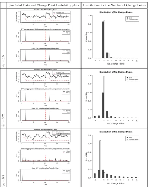
Figure 1 displays the various simulated time series and the state sequence of the underlying Markov
chain in addition to plots for the change point probabilities (left column) and the distribution of the
number of change points (right column) obtained via our proposed SMC based algorithm. The latent state
sequence is common to all of the simulated time series and is denoted by the dashed line superimposed
on the simulated time series plot.
at least 2 time periods (k= 2 ands= 1 with an ordering constraint placed upon the mean parameters) .
The change point probability (CPP) plots display the probability of switching into and out of this regime.
In all simulated time series, there are two occurrences of this regime, starting at times of approximately
20 and 120, and ending at time 100 and continuing to the end of the data, respectively.
In all three time series considered, our results indicate that our proposed methodology works well with
good detection and estimation for the change point characteristics of interest. Change point probabilities
are centred around the true locations of the starts and ends of the regime of interest with a degree of
concentration dependent upon the information contained in the data. The true number of regimes is the
most probable in all three of the time series considered.
As φ1 increases, the distribution of the change point characteristics becomes more diffuse. This is
what would be expected as the data becomes less informative as φ1 increases. This uncertainty is a
feature of the model, not a deficiency of the inferential method, and it is important to account for it
when performing estimation and prediction of related quantities. The proposed methodology is able to
do this.
We also observe that the probability that there are no change points is not negligible for φ1 = 0.75
and for φ1 = 0.90. These results illustrate the necessity of accounting for parameter uncertainty in
change point characterisation.
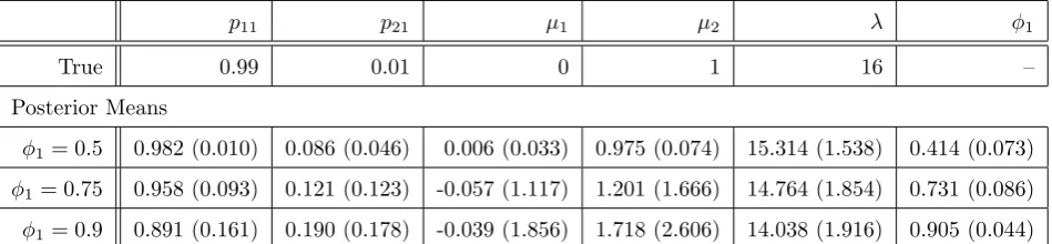
Table 1 displays the posterior means of the model parameter samples obtained via the SMC sampler.
These are calculated by taking the weighted average of the weighted cloud of samples approximating the
model parameter posterior distribution. In addition, we provide the weighted standard deviation of the
cloud of samples. We observe that the posterior values are reasonably close to the true values used to
generate the time series. We note that asφ1increases and consequently the data becomes less informative,
less accurate estimates are provided with greater deviation from the true values and commensurate
increase in standard deviation. Nevertheless, we observe that the model parameter posterior has been
reasonably well approximated.
As a comparison, we also consider the exact change point distributions obtained by conditioning on
these posterior means. We observe from the corresponding plots in Figure 1 that quite different results
can be achieved. We observe that some of the uncertainty concerning the possible additional change
points has been eliminated (see, for example, the two CPP plots when φ1 = 0.75). In addition, as
illustated by the righthand column of the figure, the distribution of the number of switches to the regime
of interest has substantially more mass on two switches having occurred. This apparently improved
confidence could be dangerously misleading in real applications.
The φ1 = 0.9 case in particular illustrates the importance of accounting for parameter uncertainty
when considering change points. We observe in the exact calculations that only one switch to the regime
of interest is the most probable which occurs at the beginning of the data, and the second occurrence
to the regime is generally not accounted for. Thus the true behaviour of the underlying system is not
p11 p21 µ1 µ2 λ φ1
True 0.99 0.01 0 1 16 –
Posterior Means
φ1= 0.5 0.982 (0.010) 0.086 (0.046) 0.006 (0.033) 0.975 (0.074) 15.314 (1.538) 0.414 (0.073)
φ1= 0.75 0.958 (0.093) 0.121 (0.123) -0.057 (1.117) 1.201 (1.666) 14.764 (1.854) 0.731 (0.086)
[image:22.595.73.548.73.183.2]φ1= 0.9 0.891 (0.161) 0.190 (0.178) -0.039 (1.856) 1.718 (2.606) 14.038 (1.916) 0.905 (0.044)
Table 1: Estimated posterior means and posterior standard deviations of parameters for the three
sim-ulated time series.
provide misleading change point conclusions and accounting for model parameter uncertainty is able to
provide an general overview with regards to different types of possible change point behaviours that
may be occurring. In Bayesian inference one should, whenever possible, base all inference upon the full
posterior distribution, marginalising out any nuisance variables and that is exactly what the proposed
method allows us to do.
4.3
fMRI Data
Functional magnetic resonance imaging (fMRI) allows the quantification of neuronal activity in-vivo
through the surrogate measurement of blood flow changes in the brain. The ability to measure these
blood flow changes relates to the so-called BOLD (blood oxygenation level dependent) effect (Ogawa
et al., 1990) where hemoglobin changes its magnetic properties dependent on whether it is carrying
oxygen or not (oxyhemoglobin and deoxyhemoglobin are diamagnetic and paramagnetic respectively).
By examining the small magnetic field changes, it is possible to quantify the relative changes in the
oxygen concentrations in the blood, which are a downstream product of neuronal activation. More
information regarding fMRI and its many inherent statistical problems can be found in Lindquist (2008).
As mentioned above, most analysis of fMRI experiments is conducted by assuming a postulated
ex-perimental design (see Worsley et al. (2002) for example) and using standard linear modelling techniques,
usually accounting for an AR component in the model. However, in many situations, it is not easy to
determine an appropriate form for the design and there is no reason to suppose a direct temporal
align-ment of the stimulus and the response. This has been shown to be particularly an issue in psychology
studies such as those on anxiety (Lindquist et al., 2007). Indeed, it will be the data from one such
ex-periment, previously analysed in Lindquist et al. (2007) which will be of interest here. In particular, we
will examine the manner in which making particular time series assumptions can affect the experimental
conclusions of the experiment and their associated uncertainty.
The data analysed in this paper comes from an anxiety inducing experiment. Below is the task
description as given in (Lindquist et al., 2007):
Simulated Data and Change Point Probability plots Distribution for the Number of Change Points φ1 = 0 . 5
0 50 100 150 200
−2
−1
0
1
2
Simulated data & Underlying Chain
Time
Sim
ulated Data
Simulated Data Underlying State Sequence
0 50 100 150 200
0.0
0.4
0.8
CPP using proposed SMC approach, accounting for parameter uncertainty
Time
CPP
P(Start) P(End)
0 50 100 150 200
0.0
0.4
0.8
Exact CPP conditioned on Posterior Mean
Time
CPP
P(Start) P(End)
0 1 2 3 4 5 6 7 8 9
10
SMC Posterior Mean Distribution of No. Change Points
No. Change Points
Probability 0.0 0.2 0.4 0.6 0.8 1.0 φ1 = 0 . 75
0 50 100 150 200
−2
−1
0
1
2
Simulated data & Underlying Chain
Time
Sim
ulated Data
Simulated Data Underlying State Sequence
0 50 100 150 200
0.0
0.4
0.8
CPP using proposed SMC approach, accounting for parameter uncertainty
Time
CPP
P(Start) P(End)
0 50 100 150 200
0.0
0.4
0.8
Exact CPP conditioned on Posterior Mean
Time
CPP
P(Start) P(End)
0 1 2 3 4 5 6 7 8 9
10
SMC Posterior Mean Distribution of No. Change Points
No. Change Points
Probability 0.0 0.2 0.4 0.6 0.8 1.0 φ1 = 0 . 9
0 50 100 150 200
−2
−1
0
1
2
Simulated data & Underlying Chain
Time
Sim
ulated Data
Simulated Data Underlying State Sequence
0 50 100 150 200
0.0
0.4
0.8
CPP using proposed SMC approach, accounting for parameter uncertainty
Time
CPP
P(Start) P(End)
0 50 100 150 200
0.0
0.4
0.8
Exact CPP conditioned on Posterior Mean
Time
CPP
P(Start) P(End)
0 1 2 3 4 5 6 7 8 9 10
SMC Posterior Mean Distribution of No. Change Points
No. Change Points
[image:23.595.71.549.66.667.2]Probability 0.0 0.2 0.4 0.6 0.8 1.0
Figure 1: Results on Simulated Data generated from a Hamilton’s MS-AR(1) model. We consider a
variety of data and display the change point probability plots and distribution of number of change
points obtained by implementing our proposed SMC based methodology. As a comparison, we also