Abstract—We construct an explicit solution for a boundary value problem for a system of partial differential equations which describes small linearized motions of three-dimensional stratified flows in the half-space. For large values of t, we obtain uniform asymptotical decompositions of the solutions on an arbitrary compact in the half-space. In the vicinity of the boundary plane, we establish the asymptotical properties of the boundary layer type: we can observe a worsening of the decay in the approximation to the bottom. The results can be used in the meteorological modelling of water flows near the bottom of the Ocean, as well as Atmosphere flows near the Earth surface. Index Terms—Atmospheric modelling and numerical prediction, boundary layer, geophysics, partial differential equations, physical oceanography, stratified fluid.
I. INTRODUCTION
We consider a system of equations of the form
1 *
1 2 *
2 3 *
3 2
* 3
3
1 2
1 2 3
0
0
0
0
0
v p
t x
v p
t x
v p
g
t x
N v
t g
v
v v
x x x
(1)
where v x t
, is a velocity field of a fluid (Ocean or Atmosphere) with components v x t1( , ) , ( , ) , ( , )v x t2 v x t3 ;( , )
p x t
is the scalar field of the dynamic pressure;
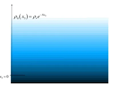
x t,is the dynamic density and *, ,g Nare positive constants. The equations (1) are deduced in [1], [2] under the assumption that the function of stationary distribution of density is performed by the exponentially decreasing
function 3
*
Nx
e
, which corresponds to the Boltzmann distribution. The system (1) can be considered as modelling Manuscript received April 20, 2019; revised July 25, 2019. This work was supported by “Programa de Investigaciones 2018-2020”, Facultad de Ciencias, Universidad de los Andes.
A. Giniatoulline is with the Department of Mathematics, Los Andes University, Cra. 1 Este No 18A-10, Bogota D. C., Colombia, South America (e-mail: [email protected]).
the linearized movement of three-dimensional fluid in a homogeneous gravitational field (Ocean or Atmosphere), as it can be visualized in the following Fig. 1:
3
) (3
Nx
e x
0
3
x
3
0 3
Nx x e
Fig. 1. Initial distribution of density as a function of x3. Some physical properties of the flows described by (1) can be found, for example, in [3]-[5].
The Cauchy problem for (1) was considered in [6], where the explicit solution was constructed and Lp -estimates were obtained. The half-space domain for (1) was considered in [7], where the solution was constructed using unilateral Fourier transform; the uniqueness of the solutions was proved in a class of growing functions, and it was established that the solution decays for large t as 1
t . The spectral
properties of the differential operator of (1) for compressible viscous case were studied in [8]. In this work, we consider the system (1) in the half-space
3 2
1
,
2,
3:
1,
2,
30
R
x x x
x x
R x
together with the initial conditions
0 0
0 0
, div 0
0
t t
v v x v
(2)
and the boundary condition
3 0
0 , 0
x
p t (3)
Without loss of generality, we may assume
* g N 1
. This can be achieved by the following change of scale, where we modify the unknown functions of
Mathematical Description of the Flows near the Bottom of
the Ocean
velocity and density and use the same notation for modified functions: v:*v , : g .
In that way, instead of system (1), we will consider the system:
1
1 2
2 3
3 3
3
1 2
1 2 3
0
0
0
0
0
v p
t x
v p
t x
v p
t x
v t
v
v v
x x x
(4)
II. CONSTRUCTION OF THE SOLUTION
To construct the solution of (4) in the half-space
R
3 , we will solve an ordinary differential equation with respect to3
x . Here we proceed in a different way if we compare it with the solution from [7], where “unilateral” sine and cosine Fouriertransforms were used with respect to x . 3
Supposing that the initial data v0
x are smooth and sufficiently well decreasing functions for x , we apply Fourier transform
x x1, 2
1, 2
and Laplace transform t
for (4). In this way, we obtain the following system:
0
1 1 1
0
2 2 2
0
3 3
3 3
3
1 1 2 2
3
ˆ 0
ˆ 0
ˆ 0
0
0
v v i P
v v i P
P
v v
x
v
v
i v i v
x
(5)
Let us denote
PP
,x3,
,
1, 2
,
12
22. In particular, for the functionP
from (5) we have the following ordinary differential equation:
0
2 2
2 3
2 2 2
3 3
ˆ
1 1 v
P
P
x x
. (6)
In terms of Fourier-Laplace transform, the boundary
condition (3) will take the form
3 0 0
x
P
. (7) We denote the characteristic roots of the equation (6) as
2 1
,
a a
.
In what follows, we will consider Re 00 . The general solution of (6) contains two arbitrary constants which depend on
and
.One of them can be defined from the condition (7), and the other - from the condition
3
lim 0
xP . In this way, we obtain
3 3
3 2
0 3 0
1 , ,
2 1
ˆ ,
a x a x
P x
v
e e d
. (8)
If we substitute the representation (8) in (5), we obtain a linear algebraic system for the functions
, 3,
, 1, 2,3 ,
, 3,
jv
x
j
x
. After solving that system, we have the following:
3 3
3 3
0
3 2
0 3 0
0 3
3 3 2 2
0 3 3
0
3 3
3
ˆ 1
, ,
2 1
ˆ
, , 1, 2,
ˆ 1
, ,
1 2 1
ˆ
Sign , ,
, , , ,
j j
j
a x a x
a x a x
v
v x
i v
e e d j
v
v x
v
e x e d
v x
x
It is easy to see that, for the inverse Fourier transform
x
, the identities hold:
2 3
2 3
1 1
2
2 3
2
1 2 2
1 3
3 3
2
2 3
2
1 1
,
1 .
x
x
F e
x x
x
x
F e
x
x
x
transform x t
will take the form:
2 3 2 3 1 1 1 2 30 0 0 0
0 1
1 1
2 2
0 1 0 1
0 1 1 , , 1 , , ; 1 1 , , 1 , ; x t x t
L F e Q k t
x
x
k Q k t J t J kt J t J k d
x
L F e R k t
x
R k t J t J kt J t J k d
(9) where J0 and J1 are Bessel functions.We use (9) and apply the inverse Fourier and Laplace transforms to (8). Thus, for the function P x t( , ) we obtain the following:
2 3 02 2 3
0 3 1 1 2 2 1 3 2 2 2 3 1 , 1 , , 4 1 , , . R x Q t
r r v
P x t dy d
x
Q t
r r
r x y x
r x y x
(10)Analogously, for the rest of the components of the solution for the problem (2)-(4), we obtain the representations:
2 0 0 0 2 0 3 3 2 2 0 0 3 1 1 0 3 3 3 2 2 2 3 2 1 1 1 , , , , 4 ,, 1, 2, 1 , , , , , 1 , , cos 1 , 1 4 1 , j j R j t
v x t v x dy Q x y t
v y d j y x Q r r
Q x y t d
x Q
r r
v x t v x t
x R t r r dy x R t r r
2 0 3 0 3 0 , , , , . R t v y dx t v x d
(11)III. ASYMPTOTICAL DECOMPOSITION ON A COMPACT SET FOR LARGE VALUES OF TIME AND BOUNDARY LAYER
PROPERTIES AT THE BOTTOM
It is easy to see that the obtained representations (10)-(11), essentially, have the same qualitative form. Thus, without loss of generality, we will investigate in detail the asymptotical behavior of one of the components of the solution. In particular, let us consider the function P x t
, .We introduce the function
30
30
3 3 3 3 1 , , 2 v v
u x x x x x
x x
.
In this way, we can represent the function P x t
, from (10), as follows:P x t
, P x t1
, P x t2
, , (12) where
3 2 3 0 3 3 1 3 32 3 3 3
1 1 , , , 4 1 1 , , , . 2 R x R
y v x y
P x t Q t dy
y y x
y
P x t dy u x y y x Q t dy
y y
We observe that P x t1
, coincides with the representation of the solution P x t
, for the Cauchy problem from [6] for the case when the initial data v0
xare extended till the whole space
R
3 . Such extension preserves the property of the solenoidality (see [9]).Now, let us consider the function P x t2
, . In other terms, we consider the function
2 3 3 3 3 3 3 3 3 0 0 2 3 2 2 2 1 , , 2 1 , , where 1 1 , sin 2. (See [6], [7]) 1 x R t y y
F x t dy f x y y x
y
Q t dy
y y
y y
Q t J t J t
y y y y
t d y y
(13)After passing in (13) to cylindrical coordinates, we obtain
3 3 0 3 21 2 3 3
0 1 , 2 , ,
cos , sin ,
x
F x t
y
Q t d
r r
dy d
f x x y x
Now, let us suppose that the function f x
satisfies the condition
3
3 2 *
1 l x , 0 1
R
x D f x dx C
l
(15)for some constants C* 0 . We introduce the notation
3 2
3 3
, : ,
h
R x x x xR x h
and observe that the internal integral with respect to
in (14) is an even function for
.We integrate by parts l +1 times in (14) with respect to 3
y and obtain thus the estimate
2 1, b l
F x t
h t
(16)
for all
t
t
00 ,
x
K
R
h3 , being K a compact. If v0
x C0
R3
then, from [6], [7] we have the uniform estimate for all
x
R
3:P x t1
, C t . (17)
To obtain the estimate (17), the expression of the main term of the asymptotic expansion was used ([10]):
1
2 2 2
1
sin
1
sin
4
, t
d
t
C O t t
t
Now, instead of studying just the main term of the asymptotic decomposition, we can consider 2l first terms.
In this way, we obtain the following estimate for 3
,
t
x
K
R
2
1 2 2
1
1 1
, cos sin
k l
k k
k l
P x t B x t B x t t
O t
(18)
We note that, for the rest of the components of the solution (11) the procedure is analogous.
Therefore, summing up (12), (16) and (18), we have proved the following result:
Theorem.
Let v0
x C2l4
R3 for some natural fixed l. Additionally, suppose that there exist positive constants Csuch that the condition holds:
3
3 2 0
1 l x , 0 2 4
R
x D v x dx C
l
.Let K be a compact such that
3 3 2
3 3
, , : ,
h h
KR R x x x xR x h .
Then, for all
h
0 ,
K
R
h3 , the asymptotic decomposition for the solution of the problem (2), (3), (4) has the following form for t :
21 2 2
1 1 0
2
1 2 2
1 1 0
, cos sin
,
, cos sin
,
k l
k k
k l
k l
k k
k l
v x t A x t A x t t
A x t O t
P x t B x t B x t t
B x t O t
,
where Aki , Bki are continuous functions on the compact K,
and there exist the positive constants a0 , b0 such that for all t t0 0 the estimate is valid:
0
00 , 2 l 1 , 0 , 2 l 1
a b
A x t B x t
h t h t
.
IV. CONCLUSION
We have studied the asymptotical behavior of the solutions of boundary value problem of the type (3) in the half-space. In other terms, we have studied the vanishing velocity of the perturbation defined by the initial data (2) for the case of the existence of an obstacle (bottom of the Ocean or the Earth surface for the case of the Atmosphere). In this process, there occurs a boundary layer-type effect in the asymptotical decompositions of the solutions for large values of t with respect to the small parameter 1
t near the plane x30. CONFLICT OF INTEREST
This work was carried out without any conflict of interest. AUTHOR CONTRIBUTIONS
As a single-author article, the research of this work, the writing of the paper and also the approval of the final version was conducted by A. Giniatoulline.
The authors would like to thank professor M. Bogovski for suggesting the topic of this article.
REFERENCES
[1] D. Tritton, Physical Fluid Dynamics, Oxford: Oxford UP, 1990. [2] P. Kundu, Fluid Mechanics, New York: Acad. Press, 1990.
[3] V. Birman and E. Meiburg, “On gravity currents in stratified ambient,”
Phys.Fluids, vol. 19, pp. 602–612, 2007.
[4] T. Dauxois and W. Young, “Near-critical reflection of internal waves,”
J.Fluid Mech., vol. 90, pp. 271–295, 1999.
[5] J. Flo, M. Ungari, and J. Bush, “Spin-up from rest in a stratified fluid: Boundary flows,” J.Fluid Mech. vol. 472, pp. 51–82, 2002.
[6] A. Giniatoulline and O. Zapata, “On some qualitative properties of stratified flows,” Contemporary Mathematics, vol. 434, pp. 193-204, 2007.
[7] A. Giniatoulline and E. Mayorga, “On some properties of the solutions of the problem modelling stratified ocean and atmosphere flows in the half-space,” Revista Colombiana Mat., vol. 41, no. 2, pp. 333–344, 2007.
[8] A. Giniatoulline and T. Castro, “On the spectrum of the operator of inner waves in a viscous compressible stratified fluid”, J. Math. Sci. Univ. Tokyo, vol. 19, pp. 313–323, 2012.
[9] V. Solonnikov, “Estimates for solutions of a non-stationary system of navier-stokes equations,” Trud Mat. Inst. Steklov, vol. 70, pp. 213-317, 1964.
[10] E. Copson, Asymptotic Expansions, Cambridge: CUP, 2004.
Copyright © 2019 by the authors. This is an open access article distributed under the Creative Commons Attribution License which permits unrestricted use, distribution, and reproduction in any medium, provided the original work is properly cited (CC BY 4.0).
Andrei Giniatoulline received his undergraduate,