ISSN: 2319-6505
DOMINANCE PREFERENTIAL REFERENCE MARKMETHOD WITH ADAPTED CLARKE & WRIGHT
HEURISTIC TO SOLVE MULTI-OBJECTIVE VEHICLE ROUTING PROBLEM
Joseph Okitonyumbe Y.F
1., Berthold Ulungu E
2., Kounhinir Some
3Joel Kapiamba NT
4and
Aristarque Ilunga K
51Mathematics Department, ISP/Mbanza-Ngungu, Democratic Republic of Congo 2LANIBIO, Université de Ouagadougou Burkina Faso
3ISTA/Kinshasa, Democratic Republic of Congo
4,5Faculty of Sciencem Université de Kinshasa, Democratic Republic of Congo
A R T I C L E I N F O A B S T R A C T
The economics heuristic of Clarke & Wright is the principle and reference model for solvingthe classical vehicle routing problem. In this paper we propose a new version of this method allowing to solve efficiently the multi-objective vehicle routing problem thanks to the preferential reference mark of dominance method. The main result is obtaining the set of efficient solutions E(P) but in a spread out way. A didactic example validates our step.
INTRODUCTION
The logistics and transports are in the center of many problems met in the industry and in the management of goods and persons. Thus, it is not surprising to see that vehicle routing problems which constitute a facet of the logistics are a part of main problems studied in operations research notably those making part of the combinatorial optimization [1]. The Vehicle Routing Problem (VRP) is a classical combinatorial optimization problem which consists to determine a set of roads for a minimal distance permitting to visit a set of customers from a central deposit (see eg [2], [3], [4], [5] and [6]). In the standard version of this problem, the fleet of vehicles is considered like being homogeneous and unlimited. It is localized in a unique disposal with autonomy allowing to serve all customers. Each vehicle has a total loading capacity of C units of products and with a limited tour duration to D units of time. Each customer i must be visited in order to deliver to him a demand ofqunits that requiresstime of service. The distancec between each couple of localizations i and j is known and symmetric. In addition to this, one supposes that the matrix of the distances respects the triangular inequality. The objective of the VRP is to minimize the covered distance by the vehicles in order to deliver the quantities asked by the customers and respecting the constraints of capacity and the different tours duration.
Therefore, many of theoretical stakes but also practical and economic are connected to this family of problems leading the existence of a lot of solving methods. Among these solving methods for Vehicle Routing Problem is the economics heuristic of Clarke and Wright. Its mono-objective version is
one of the first heuristic proposed to solve the Vehicle Routing Problem with constraint of capacity. (see [10], [11], [13]).
The economics heuristic of Clarke and Wright is very simple of application (see [7], [9], [2]). It remains a basic method that knew many variants in which the aim is, on the one hand, to improve it and on the other hand to solve other many kinds of VRP, for example the problem of Vehicles Routing Problem Time Window(VRP/TW).(see[15], [17], [18])
The aim of this work is to hybrid the economics heuristic of Clarke & Wright and the preferential reference mark of dominance method in order to solve the multiobjective vehicle routing problem [19], [20], [21]. This approach finds its interests in one of three approaches identified by Ulungu and Teghem [22], especially the methodological approach, to solve the multiobjective combinatorial optimization problems. Through this didactic example, we prove the performances of this adapted method justified by the good quality of the obtained solutions.
Thus, to present all this, we organized this paper as follows: section 2 presents mathematical formulation of the multiobjective vehicle routing problem and section, 3 present the Preferential reference mark of dominance method, 4 concerns the presentation of Clarke and Wright's economics heuristic principle. As for the multiobjective context of the economics heuristic of Clarke and Wright, it will be presented in section 5. In the following section the didactic example is solved by our adapted method. Finally, we present a
Available Online at http://journalijcar.org
International Journal
of Current Advanced
Research
International Journal of Current Advanced ResearchVol 4, Issue 10, pp 454-460, October 2015
Article History:
Received 20th, September, 2015
Received in revised form 30th, September, 2015 Accepted 13th, October, 2015 Published online 28th, October, 2015
© Copy Right, Research Alert, 2015, Academic Journals. All rights reserved.
RESEARCH ARTICLE
ISSN: 2319 - 6475
Key words:
conclusion on observations of E(P) obtainment and some issues of future research.
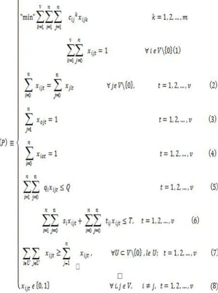
Mathematical formulation of multiobjective vehicle routing problem
Let be considered K objectives functions and v the number of delivery vehicles with a maximal capacity Q intended to serve all customers indicated by the set V from the central deposit during a maximal duration time T. The mathematical formulation of this multiobjective problem of vehicles routing is the following :
Interpretation of the different constraints of the vehicle routing problem is:
1. each customer i∈ V-\{0\} is visited one and only one time,
2. each vehicle l arriving at the customer j leaves from there.
3. and
4. each vehicle l leaving the depot comes back to it, 5. respect of the maximal capacity Q of vehicles, 6. respect of the maximal duration time T of routing, 7. elimination of the under-tours to guarantee the
connection of the different vehicle routing, 8. precise that it is a combinatorial optimization.
Solve problem (P) consists to find the entire set or part of the efficient set noted E(P)
Thus this problem raises from multiobjective combinatorial optimization. It is about to find all or a part of Pareto optimal solutions E(P). It would be illusory to solve it by using exacts methods because of its complexity. In general this complexity is coming from the number of objectives functions and/or
from the constraints and the kind of decision variables. Therefore, the use of a heuristic is required. Even since, it is a
good approximationE(P)of E(P) that we must generate.
Preferential reference mark of dominance method
Based on preference reference mark to handle dominance notion in feasible solution set of (P). interested reader can consult pages (see [23],[24],[25],[26] and [27]).
Definitions
1. Reference mark of dominance of a railable solution a is often referred to an orthonormal reference mark of origin a, dividing the space in four areas of preference in accordance to the diagram of figure 1 below.
2. Let us now consider the objectives space O of a multi-objective combinatorial optimization problem, z ,z ∈
O and V(z ) a neighborhood of z . It is said that the
solution z ∈ V(z ) certainly improves z if z is
situated in the non-dominated solutions area of the preferential reference mark of z . In this case, the acceptance probability of z equals 1. It improves z with an acceptance probability ρ, 0 < ρ< 1 when it is situated in an indifference area of the z preferential reference mark, and with a nil acceptance probability in the dominated solutions area. In other words, if ρ ≡ ℙ(acceptance of neighborhoods z of z ) then :
ρ= 1 if z ∈ III 0 < < 1 z ∈ II ∪ IV
ρ= 0 if z ∈ I
}
3. Let us consider A and B two efficient solutions of a multiobjective combinatorial optimization problem. One says the solution A is more efficient than the solution B if and only if it dominates B in the privileged direction of the decision maker.
The notion of efficiency of a solution is connected to the weights assigned to the objectives defined by the decision maker.
Stage of Dominance Preferential Reference Mark Method
Essential of this method is described on the following
Figure 1 Preferences zones in the dominance relation
Indifferencearea.
Indifference area
Dominated
solutionsarea.
I
II
IV
Non-dominated
solutions area.
III
f
1
references :(Okitonyumbe & al. 2013, 2014 and 2015). Below we present the algorithm stages.
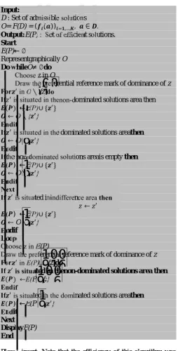
Input:
D : Set of admissible solutions
O= F(D) =( ( )) ,…, , ∈ .
Output:E(P) : Set of efficient solutions. Start
E(P)← ∅
Representgraphically O
Do whileO≠ ∅do
Choose z in O
Draw the preferential reference mark of dominance of z
For in O∖{z}do
If is situated in thenon-dominated solutions area then
( ) ←E(P)∪ { } ←O∖{ }
Endif
If is situated in the dominated solutions areathen
←O∖{ }
Endif
Ifthe non-dominated solutions areais empty then ( ) ←E(P)∪ { }
←O∖{ }
Endif Next
If is situated inindifference area then
← ( ) ←E(P)∪ { }
←O∖{ }
Endif Loop
Choose z in E(P)
Draw the preferential reference mark of dominance of z
For in E(P)∖{z}do
If is situated in thenon-dominated solutions area then ( ) ←E(P∖{z}
Endif
If is situated in the dominated solutions areathen
( ) ←E(P∖{ }
Endif Next DisplayE(P) End
Please insert: Note that the efficiency of this algorithm was discussed in (Okitonyumbe & al. 2013).
The following section is devoted to outline Clarke & Wright heuristic to be adapted for solving MOCO problem.
Clarke & Wright economics heuristic
The economics heuristic of Clarke and Wright is applied when m=1 (classical case). Its principle is based on the calculation of savings realized in uniting two partial routing or two sequences of roads [28], [7], [8]. In the initialization,
each customer i ∈ V ∖ {O}generates a road (O − i − O)
joining it by a return journey to the depot. The figure 2 shows it.
From two of these roads, for two customers i and j, it is
elementary to calculate the profitδ realized in forming only one road(O − i − j − O):
δ = c + c − c , ij ∈ V ∖ {O}, i ≠ j
This profit remains the same if two roads (O − ⋯ − i −
O)and(O − i − ⋯ − O)are merged in the road.
The initial stage of Clarke & Wright method consists to therefore calculate the matrix of saving :
δ , ij ∈ V ∖ {O}, i ≠ j
Concerning the construction of the routing, two versions are possible : the parallel version that elaborates the simultaneous different tours and the sequential version that constructs the tours one after the other.
In the two versions, once the link established between two customers, it becomes definitive. This heuristic can be considered therefore like a gluttonous heuristic. In particular:
1. In the parallel version, the profits δ are considered in the decrease order. The first tour(O − i − j − O)that is admissible, that is say verifying the capacity autonomy
constraints,…, is formed.
The process is pursued until the moment when all customers are integrated in one of the formed tours.
2. In the sequential version, in the first step, a partial tour
(O − i − j − O)is generated on basis of the biggest
admissible profit. Only the profitsδ and δ are
considered to prolong the tour either(O − k − i − j − O) or(O − i − j − l − O)with a condition, of course, these tours must remain admissible.
For each iteration, the addition of a customer in first or in last position corresponding to the biggest admissible profit is achieved until the moment when this tour cannot be prolonged without breaking the constraints. In this case, another tour is constructed with the help of the customers not yet affected.
Remark
It is noted that, the parallel version often gives better results. But a weakness of the economics heuristic of Clarke and Wright is its propensity : that is the creation of circular roads around the depot. Several attempts for remedying to that have been proposed, notably by modifying the profits :
δ ⟶δ′ = c + c −λc
with help of a parameterλto fix.
Figure 2Principe de l’heuristique de Clarke & Wright
Adaptation of the economics heuristic of Clarke and Wright to the multiobjective context
In this section, in conformity with the three proposed approaches by Ulungu and Teghem [22], we have tried to adapt the economics heuristic of Clarke and Wright to the multiobjective context.
Parameters method adjustment Savings calculation
The Savings are calculated in taking account of each objective
by using the following formula :s = c + c −
c ; i, j ∈ V\{o} ; i ≠ j, k = 1, … , m.
The realized profit by joining two segments of roads for two customers i and j in only one road (O − i − j − O)is a line matrix or column matrix of order m that assigns a value to each objective. It is the same way when one proceeds by a junction of two segments of roads
(O − ⋯ − i − O) and (O − i − ⋯ − O)into a road(O − ⋯ −
i − j − ⋯ − O).
At the initial stage of the methods, one calculates the matrix of the profits that is a tabular in which each compartment is a line matrix or column matrix of order m (see figure 2 of the paragraph 4). This tabular can be written as following :
[s ]; i, j ∈ V\{o} ; i ≠ j, k = 1, … , m.
Efficient solutions generating
The profits vector s i, j ∈ V\{o} ; i ≠ j, k = 1, … , m.
generate a cloud of points in the space. The application of the preference reference mark of dominance, as much time as necessary, produce the sets of efficient solutions by step. These different sets of efficient solutions lead us in the roads construction.
Roads Construction
There exists two methods of roads construction by economics heuristic of Clarke and Wright called parallel version and sequential version.
A. Parallel version
The profits are considered in order of efficiency in the Pareto sense and the first tour (O − i − j − O) which is admissible, that is say, verifying the constraints of capacity, of autonomy,..., is formed. The process is pursued until the moment when all customers are integrated in one of the formed tours.
B. Sequential version
After having generated at the first stage a partial tour
(O − i − j − O)on the basis of efficiency notion of the
admissible solutions, only the profits s and s are
considered for prolonging the tour
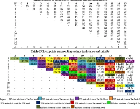
Table 1 matrix of distances in kilometers and demands in tons
N° 0 1 2 3 4 5 6 7 8 9 10 11 12 13 14 15
0 - 15 28 30 22 27 21 22 20 36 63 120 22 63 12 27
1 - 21 32 32 41 35 32 22 52 25 37 18 25 22 22
2 - 18 30 46 47 50 42 45 54 40 54 54 18 20
3 - 18 36 43 52 50 24 42 56 49 42 54 36
4 - 18 27 40 43 21 12 43 38 12 49 63
5 - 16 33 42 15 51 72 55 51 38 37
6 - 18 30 32 23 65 52 23 58 40
7 - 15 35 53 37 39 53 55 56
8 - 28 52 38 64 52 52 43
9 - 43 25 42 43 39 72
10 - 40 53 35 64 65
11 - 62 26 42 37
12 - 33 53 38
13 - 62 25
14 - 40
d - 3 3 4 2 4 2 3 4 5 3 4 2 5 4 3
Table 2 Cloud points representing savings in distance and priority
2 3 4 5 6 7 8 9 10 11 12 13 14 15
1 (22,29) (13,28) (5,27) (1,26) (1,25) (5,24) (13,23) (-1,22) (53,21) (98,20) (19,19) (53,18) (5,17) (20,16) 2 - (40,27) (20,26) (9,25) (2,24) (0,23) (6,22) (14,21) (47,20) (108,19) (-4,18) (47,17) (22,16) (35,15)
3 - - (34,25) (21,24) (8,23) (0,22) (0,21) (42,20) (51,19) (94,18) (3 ,17) (51,16) (-12,15) (21,14) 4 - - - (31,23) (16,22) (4,21) (-1,20) (37,19) (73,18) (99,17) (6,16) (73,15) (-15,14) (-14,13) 5 - - - - (32,21) (16,20) (5,19) (48,18) (39,17) (75,16) (-6,15) (39,14) (1,13) (17,12) 6 - - - (25,19)(11,18) (25,17) (61,16) (76,15) (-9,14) (61,13) (25,12) (8,11)
7 - - - (27,17) (23,16) (32,15) (105,14) (5,13) (32,12) (-21,11) (-7,10)
8 - - - (28,15) (31,14) (102,13) (-22,12) (31,11) (-20,10) (4,9)
9 - - - (56,13) (131,12) (16,11) (56,10) (-1,9) (-9,8)
10 - - - (143,11) (32,10) (91,9) (11,8) (25,7)
11 - - - (80,9) (157,8) (90,7) (110,6)
12 - - - (52,7) (-19,6) (11,5)
13 - - - (13,5) (65,4)
14 - - - (-1,3)
Legend : Efficient solutions of the first level Efficient solutions of the second level Efficient solutions of the third level Efficient solutions of the fourth level
Efficient solutions of the fifth level Efficient solutions of the sixth level Efficient solutions of the seventh level Efficient solutions of the eighth level
either (O − k − i − j − O) or (O − i − j − l − O), on condition of course these
tours remain admissible.
For each iteration, the addition of a customer in first or in last position corresponding to the biggest admissible profit
achieved until the moment when this tour can no longer be prolonged without breaking the constraints. In this case, another tour is constructed with the help of the customers not yet affected, on the basis of efficiency of savings.
Definition
Let be considered A and B two efficient solutions of a multiobjective combinatorial optimization problem, one says that the solution A is more efficient than the solution B if and only it has a bigger value that B on the privileged direction given by the decision-maker. The efficiency solution notion be bound by weights assigned to the objectives by the decision-maker.
Didactic example
A pharmaceutical industry wants to test a new product on the market. It possesses a warehouse and a fleet of vehicles with a maximum delivery capacity of 8 tons a vehicle. The demands of 15 customers are known (see tabular 1). The distances between the customers are symmetrical and verify the triangular inequality. The customers are classified according to the decrease order of priority that is encoded of 1 to 15.
Decision maker concerns
The different decision-maker concerns for organizing of the distribution routing are:
1. minimized the covered distances, 2. minimized the fleet size,
3. maximized the customers priority.
The cost is 25 UM per kilometer covered and the fixed cost of a vehicle amounts to 2500 UM.
Cloud points representing savings in distance and priority between two customers to join
In a space with two dimensions, respectively the profit in distance and in priority, we present the coordinates of partial tours visiting two customers. The dimension "size of the fleet" to minimize will intervene in roads building while respecting the capacity constraints of vehicles.
Efficient solutions
Let us note thatE(P), the set of efficient solutions obtained at the stage l, thus we have: Initially for l=1, the set of solutions potentially efficient generated by the Preferential reference
mark of dominance method is: E (P)={(22,29), (40,27),
(53,21), (98,20), (108,19), (143,11)} corresponding
respectively to the following capacity {6,7,6,7,7,7}
After suppressing of the efficient solutions of first stage, we obtain at the second stage:
E (P)={(105,14),(99,17),(94,18),(110,6),(13,28),(20,26),(3 4,25),(51,19),(47,20)}
E (P)={(10,13),(76,15),(75,16),(73,18),(5,27),(9,25),(21,24 ),(31,23),(32,21)}
E (P)={(91,9),(61,16),(53,18),(73,15),(37,19),(16,22),(8,23 ),(5,24),(1,26)}
E (P)={(89,7),(80,9),(61,13),(25,19),(14,21),(13,23),(16,20 ),(2,24),(1,25)}
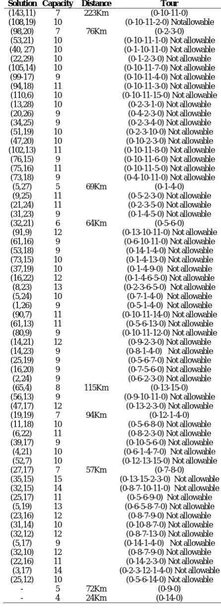
Table 3 Roads construction by the parallel version
Solution Capacity Distance Tour
(143,11) 7 223Km (0-10-11-0)
(108,19) 10 (0-10-11-2-0) Notallowable
(98,20) 7 76Km (0-2-3-0)
(53,21) 10 (0-10-11-1-0) Not allowable
(40, 27) 10 (0-1-10-11-0) Not allowable
(22,29) 10 (0-1-2-3-0) Not allowable
(105,14) 10 (0-10-11-7-0) Not allowable
(99-17) 9 (0-10-11-4-0) Not allowable
(94,18) 11 (0-10-11-3-0) Not allowable
(110,6) 10 (0-10-11-15-0) Not allowable
(13,28) 10 (0-2-3-1-0) Not allowable
(20,26) 9 (0-4-2-3-0) Not allowable
(34,25) 9 (0-2-3-4-0) Not allowable
(51,19) 10 (0-2-3-10-0) Not allowable
(47,20) 10 (0-10-2-3-0) Not allowable
(102,13) 11 (0-10-11-8-0) Not allowable
(76,15) 9 (0-10-11-6-0) Not allowable
(75,16) 11 (0-10-11-5-0) Not allowable
(73,18) 9 (0-4-10-11-0) Not allowable
(5,27) 5 69Km (0-1-4-0)
(9,25) 11 (0-5-2-3-0) Not allowable
(21,24) 11 (0-2-3-5-0) Not allowable
(31,23) 9 (0-1-4-5-0) Not allowable
(32,21) 6 64Km (0-5-6-0)
(91,9) 12 (0-13-10-11-0) Not allowable
(61,16) 9 (0-6-10-11-0) Not allowable
(53,18) 9 (0-14-1-4-0) Not allowable
(73,15) 10 (0-1-4-13-0) Not allowable
(37,19) 10 (0-1-4-9-0) Not allowable
(16,22) 12 (0-1-4-6-5-0) Not allowable
(8,23) 13 (0-2-3-6-5-0) Not allowable
(5,24) 10 (0-7-1-4-0) Not allowable
(1,26) 9 (0-5-1-4-0) Not allowable
(90,7) 11 (0-10-11-14-0) Not allowable
(61,13) 11 (0-5-6-13-0) Not allowable
(80,9) 9 (0-10-11-12-0) Not allowable
(14,21) 12 (0-9-2-3-0) Not allowable
(14,23) 9 (0-8-1-4-0) Not allowable
(25,19) 9 (0-5-6-7-0) Not allowable
(16,20) 9 (0-7-5-6-0) Not allowable
(2,24) 9 (0-6-2-3-0) Not allowable
(65,4) 8 115Km (0-13-15-0)
(56,13) 9 (0-9-10-11-0) Not allowable
(47,17) 12 (0-13-2-3-0) Not allowable
(19,19) 7 94Km (0-12-1-4-0)
(11,18) 10 (0-5-6-8-0) Not allowable
(6,22) 11 (0-8-2-3-0) Not allowable
(39,17) 9 (0-10-5-6-0) Not allowable
(4,21) 10 (0-6-1-4-7-0) Not allowable
(52,7) 10 (0-12-13-15-0) Not allowable
(27,17) 7 57Km (0-7-8-0)
(35,15) 15 (0-13-15-2-3-0) Not allowable (32,15) 14 (0-8-7-10-11-0) Not allowable
(25,17) 11 (0-5-6-9-0) Not allowable
(5,19) 13 (0-6-5-8-7-0) Not allowable
(23,16) 12 (0-8-7-9-0) Not allowable
(31,14) 10 (0-10-8-7-0) Not allowable
(32,12) 12 (0-8-7-13-0) Not allowable
(5,17) 9 (0-14-1-4-0) Not allowable
(32,10) 12 (0-8-7-9-0) Not allowable
(22,16) 11 (0-14-2-3-0) Not allowable
(3,17) 14 (0-2-3-12-1-4-0) Not allowable
(25,12) 10 (0-5-6-14-0) Not allowable
- 5 72Km (0-9-0)
E (P)={(65,4),(56,13),(37,17),(19,19),(6,22)}
E (P)={(56,10),(39,17),(4,21),(11,18)}
E (P)={(52,7),(35,15),(27,17)}
E (P)={(32,15),(25,17),(5,19)}
E (P)={(23,16),(31,14),(32,12),(5,17)}
E (P)={(32,10),(22,16),(3,17),(25,12)}
Now, we can go along to the construction of roads
Roads construction
Roads construction in Parallel method
After the execution of the three stages: E (P), E (P), E without success, we are able to notice that it remains two customers 9 and 14 when the tour (0-9-14-0) isn't allowable because it breaks the capacity constraint of the vehicles. Whence the construction of two elementary tours (0-9-0) and (0-14-0). Then, the solution obtained by the parallel version is (732,120,8) composed of eight tours : (0-10-11-0), (0-2-3-0), 5-6-0), (0,13-15-0), 12-1-4-0), 7-8-0), 9-0) and (0-14-0) and covering a total distance of 732 km with a total priority of 120.
Sequential method
The obtained solutions by the sequential version are composed of seven tours : (0-10-11-0), (0-2-3-0), (0,13-15-0), (0-12-5-6-0), (0-7-1-4-0), (0-8-14-0) and (0-9-0) whence the global cost is 37000UM and the covered distance is 780km with total priority of 120.
With a similar reasoning, by initializing the round with the solutions: (108,19), (98,20), (53,21), (40, 27) and (22,29) we obtain respectively the following solutions :
1. Solution: (833, 120,8) corresponding to the rounds: (0-2-11-0), (0-1-10-0), (0-2-3-0), (0-7-12-15-0), (0-5-6-0), (0-8-14-0), (0-9-0) and (0-13-0) .
2. Solution: (745, 120,8) conforms to the rounds: (0-1-11-0), (0-2-3-(0-1-11-0), (0-4-5-(0-1-11-0), (0-12-13-(0-1-11-0), (0-7-6-10-(0-1-11-0), (0-8-15-0), (0-9-0) and (0-14-0).
3. Solution: (754, 120,8) appropriate with the rounds: 1-10-0), 2-3-0), 4-11-0), 5-6-0), 7-8-0), (0-12-13-0), (0-14-15-0) and (0-9-0).
4. Solution: (754, 120, 8)corresponding with the Rounds: (0-2-3-0), (0-1-10-0), (0-4-11-0), (0-5-6-0), (0-7-8-0), (0-12-13-0), (0-14-15-0) and (0-9-0).
5. Solution: (862, 120, 8) conforms to the rounds: (0-1-2-0), (0-10-11-(0-1-2-0), (0-5-6-(0-1-2-0), (0-7-8-(0-1-2-0), (0-12-13-(0-1-2-0), (0-14-15-0) and (0-9-0).
RESULTS AND DISCUSSION
The obtained solutions by the sequential method are : (780,120,7), (833,120,8), (745,120,8)$, $(754,120,8) and (862,120,8) but the decision maker choice must be worked on two solutions : (780,120,7) and (745,120,8$ because the other are dominated. If it were asked to us to give a point of view to the decision maker, it is the first solution which we would have advised to choose because the additional cost generated by the increase of the distance that is 35 Km X 25 Um/Km = 875 Um is negligible compared to the fixed cost of a vehicle which amounts to 2500 UM.
CONCLUSION AND PERSPECTIVES
As the most used of heuristics in multiobjective optimization, the economics heuristic of Clark and Wright is dedicated to mono-objective optimization. This work is the best adaptation of this heuristic to multiobjective optimization. Through the didactic example of the results obtained above we see that this adaptive method is the best method to solve the multiobjective vehicles routing problems with an unlimited fleet and unique depot. Besides we have proved, in this paper that, the sequential version gave the better result than the parallel version in the multiobjective context, that is the contrary in mono-objective.
It is also necessary to add the fact that the sequential version permitted us to get these solutions in nine iterations whereas the parallel version drove us until sixty-five iterations creating thus several circular roads around the depot. Indeed, it reduced the size of the fleet to seven vehicles while keeping the same total priority than the parallel version. In the future works we will try to program the sequential version of this multiobjective version of economics heuristic of Clarke and Wright in order to solve lots of problems.
References
1. Okitonyumbe Y.F. and Ulungu E.-L., Nouvelle caractérisation des solutions efficaces des problèmes
d'optimisation combinatoire multi-objectif, Revu
Congolaise des Sciences nucléaires, Volume 27, pp 47-61, décembre, 2013.
2. Laporte, G., Semet F.,Classical heuristics for the capacitated VRP, The Vehicle Routing Problem, P. Toth et D. Vigo (éditeurs), SIAM Monographs on Discrete
Mathematics and Applications, pp : 109-128,
Philadelphia 2002.
3. Solomon, M. M.,"Algorithms for the vehicle routing and
scheduling problems with time window constraints,”
Operations Research, vol. 35, no. 2, pp. 254–265, 1987. 4. Thangiah, R., Nygard, K. E. and Juell, P. L.,"GIDEON:
a genetic algorithm system for vehicle routing with time
windows,” in Proceedings of the 7th IEEE Conference
on Artificial Intelligence Applications, pp. 322–328, Miami Beach, Fla, USA, February 1991.
5. Ombuki, B., Ross, B. J. and Hanshar, F., "Multi-objective genetic algorithm for vehicle routing problem
with time windows,” Applied Intelligence, vol. 24, pp.
17–33, 2006.
Table 4
Solution Capacity Distance Tour
(143,11) 7 223Km (0-10-11-0)
(98,20) 7 64Km (0-2-3-0)
(65,4) 8 115KM (0-13-15-0)
(32,21) 6 (0-5-6-0)
(-6,15) 8 114Km (0-12-5-6-0)
(5,27) 5 (0-1-4-0)
(5,24) 8 108Km (0-7-1-4-0)
(-20,10) 8 84Km (0-8-14-0)
6. Figliozzi, M. A.,"An iterative route construction and improvement algorithm for the vehicle routing problem
with soft time windows,”Transportation Research C,
vol. 18, no. 5, pp. 668–679, 2010.
7. Teghem, J., Recherche opérationnelle Tome2 : Gestion de production, Modèles aléatoire et Aide multicritère, Ellipses 2013.
8. Teghem, J., Recherche opérationnelle Tome1: Méthodes d'optimisation, Ellipses 2012.
9. Das I., Dennis J.,A closer look at drawbacks of minimising weighted sum of multiobjective for Pareto set generation in multicriteria optimisation problems, structural optimization, 14 : pp 63-69, 1997.
10.Thangiah, S.,“Vehicle routing with time windows using
genetic algorithms,” in Applications Handbook of
Genetic Algorithms: New Frontiers, Volume II, pp.
253–277, CRC Press, Boca Raton, Fla, USA, 1995.
11.Jozefowiez, N., Semet, F. and Talbi, E.,“Target aiming
Pareto search and its application to the vehicle routing
problem with route balancing,” Journal of Heuristics,
vol. 13, no. 5, pp. 455–469, 2007.
12.Alvarenga, G. B., Mateus, G. R. and de Tomi, G.,“A
genetic and set partitioning two-phase approach for the
vehicle routing problem with time windows,”
Computers and Operations Research, vol. 34, no. 6, pp.
1561–1584, 2007.
13.Jozefowiez,N., Semet, F. and Talbi, E.,“Multi-objective
vehicle routing problems,” European Journal of
Operational Research, vol. 189, no. 2, pp. 293–309,
2008.
14.Pang, K.,“An adaptive parallel route construction
heuristic for the vehicle routing problem with time
windows constraints,” Expert Systems with
Applications, vol. 38, no. 9, pp. 11939–11946, 2011.
15. Ghoseiri, K. and Ghannadpour, S. F.,“Multi-objective vehicle routing problem with time windows using goal
programming and genetic algorithm,” Applied Soft
Computing Journal, vol. 10, no. 4, pp. 1096–1107,
2010.
16.Tan, K. C., Lee, L. H., Zhu, Q. L. and Ou, K.,“Heuristic
methods for vehicle routing problem with time
windows,” Artificial Intelligence in Engineering, vol.
15, no. 3, pp. 281–295, 2001.
17.Chiang, W. and Russell, R. A.,“Simulated annealing
metaheuristics for the vehicle routing problem with time
windows,” Annals of Operations Research, vol. 63, pp. 3–27, 1996.
18. Taillard, E. D., Badeau, P., Gendreau, M., Guertin, F.
and Potvin, J.,“A tabu search heuristic for the vehicle routing problem with soft time windows,”
Transportation Science, vol. 31, no. 2, pp. 170–186,
1997.
19. Tan, K. C., Chew, Y. H. and Lee, L. H.,“A hybrid
multiobjective evolutionary algorithm for solving
vehicle routing problem with time windows,”
Computational Optimization and Applications, vol. 34, no. 1, pp. 115–151, 2006.
20. Thangiah,S. R.,“A hybrid genetic algorithms, simulated
annealing and tabu search heuristic for vehicle routing
problems with time windows,” in Practical Handbook of
Genetic Algorithms Complex Structures, Volume 3. L.
Chambers, pp. 374–381, CRC Press, 1999.
21. Tan,, K. C., Lee, L. H. and K. Ou,“Hybrid genetic
algorithms in solving vehicle routing problems with
time window constraints,” Asia-Pacific Journal of
Operational Research, vol. 18, no. 1, pp. 121–130,
2001.
22. Ulungu E. L. and Teghem, J.,Multi-objective
Combinatorial Optimization Problem : A survey.
Journal of Multicriteria Decision Analysis, 3, pp
83-104, 1994.
23. Okitonyumbe Y.F.,Optimisation combinatoire multi-objectif : méthodes exactes et Metaheuristiques, mémoire de DEA de mathématiques appliquées, Université Pédagogique Nationale, R.D. Congo, Septembre 2012.
24. Okitonyumbe Y.F. and Ulungu E.-L., Résolution du problème multi-objectif de tournées de distribution par
l’algorithme de toile d’araignées, REBUTO-RDC, Numéro 41, pp 33-46, décembre 2014.
25. Okitonyumbe Y.F. and Ulungu E.-L., Résolution des problèmes multi-objectifs d’affectation et de sac-à-dos par la m'méthode du repèrepréférentiel de dominance, REBUTO-RDC, Numéro 41, pp 105-118, décembre 2014.
26. Okitonyumbe Y.F., Berthold Ulungu E.-L. Joël KAPIAMBA Nt., Résolution du problème multi-objectif
de tournées de véhicules par l’heuristique de Clarke et
Wright, Centre de Recherche Inter Disciplinaire de l'UniversitéPédagogique Nationale , (under press) 2015. 27. Okitonyumbe Y.F. and Ulungu E.-L.,Cobweb Heuristic
for solving the Multi-Objective Vehicle Routing
Problem, in International Journal of Applied
Mathematical Research, Vol. 4 numéro 3 pp 430-436,
2015.
28. Clarke G., Wright J.V., Scheduling of vehicles from a central depot to a number of delivery point, Operation Research 12 : pp 568-581, 1964.