Point And Density Forecasts In Panel Data Models

University of Pennsylvania

ScholarlyCommons

Publicly Accessible Penn Dissertations

2017

Point And Density Forecasts In Panel Data Models

Laura Liu

University of Pennsylvania, yuliu4@sas.upenn.edu

Follow this and additional works at:

https://repository.upenn.edu/edissertations

Part of the

Economics Commons

This paper is posted at ScholarlyCommons.https://repository.upenn.edu/edissertations/2432

For more information, please contactrepository@pobox.upenn.edu.

Recommended Citation

Liu, Laura, "Point And Density Forecasts In Panel Data Models" (2017).Publicly Accessible Penn Dissertations. 2432.

Point And Density Forecasts In Panel Data Models

Abstract

This dissertation develops econometric methods that facilitate estimation and improve forecasting

performance in panel data models. The panel considered in this paper features large cross-sectional dimension (N) but short time series (T). It is modeled by a dynamic linear model with common and heterogeneous coefficients and cross-sectional heteroskedasticity. Due to short T, traditional methods have difficulty in disentangling the heterogeneous parameters from the shocks, which contaminates the estimates of the heterogeneous parameters. To tackle this problem, the methods developed in this dissertation assume that there is an underlying distribution of the heterogeneous parameters and pool the information from the whole cross-section together via this distribution. Chapter 2, coauthored with Hyungsik Roger Moon and Frank Schorfheide, constructs point forecasts using an empirical Bayes method that builds on Tweedie's formula to obtain the posterior mean of the heterogeneous coefficients under a correlated random effects distribution. We show that the risk of a predictor based on a non-parametric estimate of the Tweedie correction is asymptotically equivalent to the risk of a predictor that treats the correlated-random-effects distribution as known (ratio-optimality). Our empirical Bayes predictor performs well compared to various competitors in a Monte Carlo study. In an empirical application, we use the predictor to forecast revenues for a large panel of bank holding companies and compare forecasts that condition on actual and severely adverse macroeconomic conditions. In Chapter 3, I focus on density forecasts and use a full Bayes approach, where the distribution of the heterogeneous coefficients is modeled nonparametrically allowing for correlation between heterogeneous parameters and initial conditions as well as individual-specific regressors. I develop a simulation-based posterior sampling algorithm specifically addressing the nonparametric density estimation of unobserved heterogeneous parameters. I prove that both the estimated common parameters and the estimated distribution of the heterogeneous parameters achieve posterior consistency, and that the density forecasts asymptotically converge to the oracle forecast. Monte Carlo simulations and an application to young firm dynamics demonstrate improvements in density forecasts relative to alternative approaches.

Degree Type Dissertation

Degree Name

Doctor of Philosophy (PhD)

Graduate Group Economics

First Advisor Francis X. Diebold

Keywords

Bank Stress Tests, Bayesian, Density Forecasts, Panel Data, Point Forecasts, Young Firms Dynamics

POINT AND DENSITY FORECASTS IN PANEL DATA MODELS

Laura Liu

A DISSERTATION

in

Economics

Presented to the Faculties of the University of Pennsylvania

in

Partial Fulllment of the Requirements for the

Degree of Doctor of Philosophy

2017

Supervisor of Dissertation

Francis X. Diebold Professor of Economics

Co-Supervisor of Dissertation

Frank Schorfheide Professor of Economics

Graduate Group Chairperson

Jesús Fernández-Villaverde Professor of Economics

Dissertation Committee

Francis X. Diebold, Professor of Economics Frank Schorfheide, Professor of Economics Xu Cheng, Associate Professor of Economics

POINT AND DENSITY FORECASTS IN PANEL DATA MODELS

c

COPYRIGHT

2017

Yu Liu

This work is licensed under the Creative Commons Attribution NonCommercial-ShareAlike 3.0 License

To view a copy of this license, visit

ACKNOWLEDGEMENT

I am immensely indebted to my advisors, Francis X. Diebold and Frank Schorfheide, and other members of my committee, Xu Cheng and Francis J. DiTraglia. Their interesting lectures in the rst year triggered my compassion in econometrics. As I went from the courses to the research, their invaluable advice and support guided me through step by step. Looking back, I cannot imagine myself making such progress and completing this dissertation without them. It is a blessing to have professors as insightful and caring as them, who are also role models for my future endeavor as an economist.

I am grateful to many other professors for their great lectures that broaden my view of economics and their patience with my every naive question. In particular, I greatly bene-ted from helpful discussions with Timothy Christensen, Benjamin Connault, and Jeremy Greenwood.

I would like to express my appreciation to my coauthors, Mert Demirer, Maria Grith, Chris-tian Matthes, Hyungsik Roger Moon, Katerina Petrova, Kamil Yilmaz, and Molin Zhong. I have learned a lot from them beyond the scope of the projects, and hard work has become enjoyable experiences thanks to them.

I would like to thank all my friends, classmates, and everyone in the econometrics group. Thanks to Yunan Li for being my best friend since the rst year of graduate school. Thanks to Nicolas Janetos, Ami Ko, and Jan Tilly for the good time and space we shared together and the support both in research and in life. Thanks to Ross Askanazi, Lorenzo Braccini, Minsu Chang, Pengfei Han, Yang Liu, Paul Sangrey, Minchul Shin, and Jacob Warren for all the thought-provoking conversations on econometrics and economics in general.

ABSTRACT

POINT AND DENSITY FORECASTS IN PANEL DATA MODELS

Laura Liu

Francis X. Diebold Frank Schorfheide

This dissertation develops econometric methods that facilitate estimation and improve fore-casting performance in panel data models. The panel considered in this paper features large cross-sectional dimension (N) but short time series (T). It is modeled by a dynamic

linear model with common and heterogeneous coecients and cross-sectional heteroskedas-ticity. Due to shortT, traditional methods have diculty in disentangling the heterogeneous

TABLE OF CONTENTS

Acknowledgement . . . iii

Abstract . . . v

List of Tables . . . x

List of Illustrations . . . xi

CHAPTER 1 : Introduction . . . 1

CHAPTER 2 : Point Forecasts and Bank Stress Tests . . . 5

2.1 Introduction . . . 5

2.2 A Dynamic Panel Forecasting Model . . . 11

2.3 Decision-Theoretic Foundation . . . 15

2.4 Implementation of the Optimal Forecast . . . 20

2.5 Ratio Optimality in the Basic Dynamic Panel Model . . . 27

2.6 Monte Carlo Simulations . . . 31

2.7 Empirical Application . . . 43

2.8 Conclusion . . . 54

CHAPTER 3 : Density Forecasts and Young Firm Dynamics . . . 55

3.1 Introduction . . . 55

3.2 Model . . . 63

3.3 Numerical Implementation . . . 71

3.4 Theoretical Properties . . . 79

3.5 Extensions . . . 93

3.6 Simulation . . . 105

3.8 Concluding Remarks . . . 125

APPENDIX A : Point Forecasts and Bank Stress Tests . . . 127

A.1 Theoretical Derivations and Proofs . . . 127

A.2 Data Set . . . 176

A.3 Additional Empirical Results . . . 180

APPENDIX B : Density Forecasts and Young Firm Dynamics . . . 181

B.1 Notations . . . 181

B.2 Algorithms . . . 182

B.3 Proofs for Baseline Model . . . 192

B.4 Proofs for General Model . . . 209

B.5 Extension: Heavy Tails . . . 216

B.6 Simulations . . . 217

LIST OF TABLES

TABLE 1 : Monte Carlo Design 1 . . . 32

TABLE 2 : Monte Carlo Experiment 1: Random Eects, Parametric Tweedie Correction, Selection Bias . . . 34

TABLE 3 : Monte Carlo Design 2 . . . 37

TABLE 4 : Monte Carlo Experiment 2: Correlated Random Eects, Non-parametric versus Parametric Tweedie Correction . . . 41

TABLE 5 : Monte Carlo Design 3 . . . 42

TABLE 6 : Monte Carlo Experiment 3: Misspecied Likelihood Function . . . . 43

TABLE 7 : MSE for Basic Dynamic Panel Model . . . 45

TABLE 8 : MSE for Basic Dynamic Panel Model forT = 5 . . . 47

TABLE 9 : Parameter Estimates for T = 5: θˆQM LE, Parametric Tweedie Cor-rection . . . 48

TABLE 10 : MSE for Model with Unemployment forT = 5 . . . 50

TABLE 11 : MSE for Model with Unemployment, Fed Funds Rate, and Spread for T = 11 . . . 52

TABLE 12 : Simulation Setup: Baseline Model . . . 108

TABLE 13 : Forecast Evaluation: Baseline Model . . . 111

TABLE 14 : Simulation Setup: General Model . . . 114

TABLE 15 : Prior Structures . . . 115

TABLE 16 : Forecast Evaluation: General Model . . . 117

TABLE 17 : Descriptive Statistics for Observable . . . 119

TABLE 18 : Common Parameterβ . . . 120

TABLE 19 : Forecast Evaluation: Young Firm Dynamics . . . 122

LIST OF ILLUSTRATIONS

FIGURE 1 : QMLE Estimation: Distribution ofEbλi_ˆ θ,Yi

[λi]versusλˆi(ˆθ) . . . 36

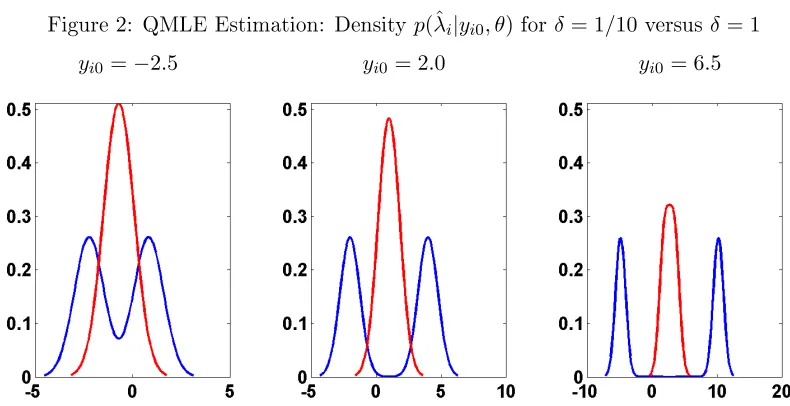
FIGURE 2 : QMLE Estimation: Densityp(ˆλi|yi0, θ)for δ = 1/10 versusδ = 1. . 37

FIGURE 3 : QMLE Estimation: True Densityp(ˆλi|yi0, θ)versus Gaussian and Nonparametric Estimates . . . 39

FIGURE 4 : QMLE Estimation: Gaussian versus Nonparametric Estimates Tweedie Correction . . . 40

FIGURE 5 : Tweedie Corrections forT = 5 and τ = 2012 . . . 46

FIGURE 6 : Predictions under Actual and Stressed Scenario forT = 5 . . . 51

FIGURE 7 : Predictions under Actual and Stressed Scenario for T = 11 and τ = 2013 . . . 53

FIGURE 8 : f0 vsΠ (f |y1:N,0:T) : Baseline Model . . . 112

FIGURE 9 : DGP: General Model . . . 115

FIGURE 10 : Histograms for Observables . . . 119

FIGURE 11 : PIT . . . 123

FIGURE 12 : Predictive Distributions: 10 Randomly Selected Firms . . . 123

FIGURE 13 : Predictive Distributions: Aggregated by Sectors . . . 124

FIGURE 14 : Joint Distributions of_λˆ_{i and Condition Variable . . . 126}

FIGURE 15 : Convergence Diagnostics: β. . . 218

FIGURE 16 : Convergence Diagnostics: σ2 . . . 219

FIGURE 17 : Convergence Diagnostics: α . . . 220

FIGURE 18 : Convergence Diagnostics: λ1 . . . 221

CHAPTER 1

Introduction

This dissertation develops econometric methods that facilitate estimation and improve fore-casting performance in panel data models. Panel data, such as a collection of rms or house-holds observed repeatedly for a number of periods, are widely used in empirical studies and can be useful for forecasting individuals' future outcomes, which is interesting and impor-tant in many cases. For example, in the context of banks, stress tests involve forecasting pre-provision net revenues (PPNR) and other balance sheet variables under counterfactual stressed macroeconomic and nancial scenarios; in the context of young rms, accurate forecasts can help investors select promising startups and assist policymakers in regulating entrepreneur funding.

For illustrative purposes, let us consider a simple dynamic panel data model:

yit=βyi,t−1+λi+uit, uit∼N 0, σ2

,

where i = 1,· · ·, N, and t = 1,· · · , T + 1. The yit's are observed individual outcomes,

β and σ2 are common parameters, and λi's are unobserved individual eects. The general model studied in this dissertation extends this baseline setup to account for many important features of real-world empirical studies, including regressors with common eects, correlated random coecients, and cross-sectional heteroskedasticity. Based on the observed panel up to timeT, I am interested in providing point and density forecasts of yi,T+1.

The panel considered in this paper features large cross-sectional dimension (N) but short

time series (T). This framework is appealing to the bank stress tests example due to changes

number of observations for each young rm is restricted by its age.

Due to short T, traditional methods have diculty in disentangling the unobserved

indi-vidual eects from the shocks, which contaminates the estimates of the indiindi-vidual eects. The naive estimators that only utilize the individual-specic observations are inconsistent even if N goes to innity. To tackle this problem, the methods developed in this

disserta-tion assume that there is an underlying distribudisserta-tion of the individual eects. Moreover, the individual eects are allowed to be correlated with the initial condition yi0, i.e. correlated random eects model. Then, we can pool the information from the whole cross-section to-gether via this distribution in an ecient and exible way, and provide better estimates of the individual eects and more accurate forecasts of the individual-specic future outcomes.

The methods proposed in this dissertation are general to many other problems beyond fore-casting. Here estimating heterogeneous parameters is important because we want to generate good forecasts, but in other cases, the heterogeneous parameters themselves can possibly be the objects of interest. For example, people may be interested in individual-specic treatment eects, and the technique developed here can be applied to those questions.

Chapter 2, coauthored with Hyungsik Roger Moon and Frank Schorfheide, constructs point forecasts using an empirical Bayes method that builds on Tweedie's formula to obtain the posterior mean of the heterogeneous coecients under a correlated random eects distribu-tion. This formula utilizes cross-sectional information to transform the unit-specic (quasi) maximum likelihood estimator into an approximation of the posterior mean under a prior distribution that equals the population distribution of the random coecients.

Our empirical Bayes predictor performs well compared to various competitors in a Monte Carlo study. In an empirical application, we use the predictor to forecast revenues for a large panel of bank holding companies and compare forecasts that condition on actual and severely adverse macroeconomic conditions. Results show that the impact of stressed macroeconomic conditions (characterized by unemployment, federal funds rate, and spread) on bank revenues is relatively small with respect to the cross-sectional dispersion of revenues.

In Chapter 3, I tackle a dierent problem in a similar panel data setup as described in Chapter 2. Instead of providing point forecasts via an empirical Bayes method, here I focus on density forecasts and use a full Bayes approach, where the distribution of the heterogeneous coecients is modeled nonparametrically by a mixture model allowing for correlation between heterogeneous parameters and initial conditions as well as individual-specic regressors. Once this distribution is estimated by exploring the information from the whole cross-section, I can, intuitively speaking, use it as a prior distribution and combine it with specic data and obtain the specic posterior. This individual-specic posterior helps provide better inference about the heterogeneous parameters of each individual.

In this framework, it is natural to construct density forecasts. Basically, it is a predictive distribution of future performance of a specic rm, which summarizes all sources of future uncertainties. Especially, in this setup of dynamic panel data model, the density forecasts reect uncertainties due to future shocks, individual heterogeneity, and estimation uncer-tainty, where the part of uncertainties due to individual heterogeneity arises from the lack of time-series information available to infer the heterogeneous parameters of each individ-ual. Moreover, based on density forecasts, it is straightforward to derive point forecasts and interval forecasts.

pa-rameters achieve posterior consistency, and that the density forecasts asymptotically con-verge to the oracle forecast, an (infeasible) benchmark that is dened as the individual-specic posterior predictive distribution under the assumption that the common parameters and the distribution of the heterogeneous parameters are known.

CHAPTER 2

Point Forecasts and Bank Stress Tests

1

2.1 Introduction

The main goal of this paper is to forecast a collection of short time series. Examples are the performance of start-up companies, developmental skills of small children, and revenues and leverage of banks after signicant regulatory changes. In these applications the key diculty lies in the ecient implementation of the forecast. Due to the short time span, each time series taken by itself provides insucient sample information to precisely estimate unit-specic parameters. We will use the cross-sectional information in the sample to make inference about the distribution of heterogeneous parameters. This distribution can then serve as a prior for the unit-specic coecients to sharpen posterior inference based on the short time series.

More specically, we consider a linear dynamic panel model in which the unobserved in-dividual heterogeneity, which we denote by the vector λi, interacts with some observed predictors:

Yit=λ0iWit−1+ρ0Xit−1+α0Zit−1+Uit, i= 1, . . . , N, t= 1, . . . , T. (2.1.1) Here, (Wit−1, Xit−1, Zit−1) are predictors and Uit is an unpredictable shock. Throughout this paper we adopt a correlated random eects approach in which the λis are treated as random variables that are possibly correlated with some of the predictors. An important special case is the linear dynamic panel data model in whichWit−1= 1,λiis a heterogeneous intercept, and the sole predictor is the lagged dependent variable: Xit−1 =Yit−1.

We develop methods to generate point forecasts ofYiT+1, assuming that the time dimension

T is short relative to the number of predictors(WiT, XiT, ZiT). The forecasts are evaluated under a quadratic loss function. In this setting an accurate forecasts not only requires a precise estimate of the common parameters (α, ρ), but also of the parameters λi that are specic to the cross-sectional unitsi. The existing literature on dynamic panel data models

almost exclusively studied the estimation of the common parameters, treating the unit-specic parameters as a nuisance. Our paper builds on the insights of the dynamic panel literature and focuses on the estimation ofλi, which is essential for the prediction ofYit. The benchmark for our prediction methods is the so-called oracle forecast. The oracle is assumed to know the common coecients (α, ρ) as well as the distribution of the heteroge-neous coecients λi, denoted by π(λi|·). Note that this distribution could be conditional on some observable characteristics of unit i. Because we are interested in forecasts for the

entire cross section of N units, a natural notion of risk is that of compound risk, which is

a (possibly weighted) cross-sectional average of expected losses. In a correlated random-eects setting, this averaging is done under the distribution π(λi|·), which means that the compound risk associated with the forecasts of theN units is the same as the integrated risk

for the forecast of a particular uniti. It is well known, that the integrated risk is minimized

by the Bayes predictor that minimizes the posterior expected loss conditional on time T

information for uniti. Thus, the oracle replacesλi by its posterior mean.

gener-alized method of moments (GMM) estimator, a likelihood-based correlated random eects estimator, or a Bayes estimator.

Our paper makes three contributions. First, we show in the context of the linear dynamic panel data model that a feasible predictor based on a consistent estimator of (ρ, α) and a non-parametric estimator of the cross-sectional density of the relevant sucient statistics can achieve the same compound risk as the oracle predictor asymptotically. Our main theorem extends a result from Brown and Greenshtein (2009) for a vector of means to a panel data model with estimated common coecients. Importantly, this result also covers the case in which the distribution π(λi|·) degenerates to a point mass. As in Brown and Greenshtein (2009), we are able to show that the rate of convergence to the oracle risk accelerates in the case of homogeneous λcoecients. Second, we provide a detailed Monte Carlo study that

compares the performance of various implementations, both non-parametric and parametric, of our predictor. Third, we use our techniques to forecast pre-provision net-revenues of a panel of banks.

If the time series dimension is small, our feasible predictor performs much better than a naive predictor of YiT+1 that is based on within-group estimates of λi. A small T leads to a noisy estimate of λi. Moreover, from a compound risk perspective, there will be a selection bias. Consider the special case of α = ρ = 0 and Wit = 1. Here, λi is simply a heterogeneous intercept. Very large (small) realizations of Yit will be attributed to large (small) values of λi, which means that the within-group mean will be upward (downward) biased for those units. The use of a prior distribution estimated from the cross-sectional information essentially corrects this bias, which facilitates the reduction of the prediction risk if it is averaged over the entire cross section. Alternatively, one could ignore the cross-sectional heterogeneity and estimate a (misspecied) model with a homogeneous coecient

λ. If the heterogeneity is small, this procedure is likely to perform well in a

implementations of the feasible predictor in a Monte Carlo study and provide comparisons with other predictors, including one that is based on quasi maximum likelihood estimation of the unit-specic coecients and one that is constructed from a pooled OLS estimator that ignores parameter heterogeneity.

In an empirical application we forecast pre-provision net revenues of bank holding companies. The stress tests that have become mandatory under the Dodd-Frank Act require banks to establish how revenues vary in stressed macroeconomic and nancial scenarios. We capture the eect of macroeconomic conditions on bank performance by including the unemployment rate, an interest rate, and an interest rate spread in the vector Wit−1 in (2.1.1). Our analysis consists of two steps. We rst document the one-year-ahead forecast accuracy of the posterior mean predictor developed in this paper under the actual economic conditions, meaning that we set the aggregate covariates to their observed values. In a second step, we replace the observed values of the macroeconomic covariates by counterfactual values that reect severely adverse macroeconomic conditions. We nd that our proposed posterior mean predictor is considerably more accurate than a predictor that does not utilize any prior distribution. The posterior mean predictor shrinks the estimates of the unit-specic coecients toward a common prior mean, which reduces its sampling variability. According to our estimates, the eect of stressed macroeconomic conditions on bank revenues is very small relative to the cross-sectional dispersion of revenues across holding companies.

Robbins (1956) (see Robert (1994) for a textbook treatment).

We use compound decision theory as in Robbins (1964), Brown and Greenshtein (2009), Jiang and Zhang (2009) to state our optimality result. Because our setup nests the linear dynamic panel data model, we utilize results on the consistent estimation of ρ in dynamic

panel data models with xed eects when T is small, e.g., Anderson and Hsiao (1981),

Arellano and Bond (1991), Arellano and Bover (1995), Blundell and Bond (1998), Alvarez and Arellano (2003). Fully Bayesian approaches to the analysis of dynamic panel data models have been developed in Chamberlain and Hirano (1999), Hirano (2002), Lancaster (2002).

The papers that are most closely related to ours are Gu and Koenker (2016a,b). They also consider a linear panel data model and use Tweedie's formula to construct an approximation to the posterior mean of the heterogeneous regression coecients. However, their papers focus on the use of the Kiefer-Wolfowitz estimator for the cross-sectional distribution of the sucient statistics, whereas our paper explores various plug-in estimators for the homo-geneous coecients in combination with both parametric and nonparametric estimates of the cross-sectional distribution. Moreover, our paper establishes the ratio-optimality of the forecast and presents a dierent application. Finally, Liu (2016) develops a fully Bayesian (as opposed to empirical Bayes) approach to construct density forecast. She uses a Dirichlet process mixture to construct a prior for the distribution of the heterogeneous coecients, which then is updated in view of the observed panel data.

distributions. Second, the BLUP method nds the forecast that minimizes the expected quadratic loss in the class of linear (in (Yi0, ..., YiT)0) and unbiased forecasts. Therefore, it is not necessarily optimal in our framework that constructs the optimal forecast without restricting the class of forecasts. Third, the existing panel forecasts based on the BLUP were developed for panel regressions with random eects and do not apply to correlated random eects settings.

There is a small academic literature on econometric techniques for stress test. Most papers analyze revenue and balance sheet data for the relatively small set of bank holding companies with consolidated assets of more than 50 billion dollars. There are slightly more than 30 of these companies and they are subject to the Comprehensive Capital Analysis and Review conducted by the Federal Reserve Board of Governors. An important paper in this literature is Covas et al. (2014), which uses quantile autoregressive models to forecast bank balance sheet and revenue components. We work with a much larger panel of bank holding companies that comprises, depending on the sample period, between 460 and 725 institutions.

2.2 A Dynamic Panel Forecasting Model

We consider a panel with observations for cross-sectional units i = 1, . . . , N in periods t= 1, . . . , T. Observation Yit is assumed to be generated by (2.1.1). We distinguish three types of regressors. First, thekw×1vectorWit interacts with the heterogeneous coecients

λi. In many panel data applications Wit = 1, meaning that λi is simply a heterogenous intercept. We allow Wit to also include deterministic time eects such as seasonality, time trends and/or strictly exogenous variables observed at timet. To distinguish deterministic

time eects w1,t+1 from cross-sectionally varying and strictly exogenous variablesW2,it, we partition the vector into Wit = (w1,t+1, W2,it).2 The dimensions of the two components are kw1 and kw2, respectively. Second, Xit is a kx ×1 vector of sequentially exogenous predictors with homogeneous coecients. The predictorsXit may include lags ofYit+1 and we collect all the predetermined variables other than the lagged dependent variable into the subvectorX2,it. Third,Zit is akz-vector of strictly exogenous regressors, also with common coecients.

Our main goal is to construct optimal forecasts of (Y1T+1, ..., YN T+1) conditional on the entire panel observations {(Yit, Wit−1, Xit−1, Zit−1),i= 1, . . . , N and t= 1, ..., T using the forecasting model (2.1.1). An important special case of model (2.1.1) is the basic dynamic panel data model

Yit=λi+ρYit−1+Uit, (2.2.1) which is obtained by setting Wit = 1, Xit = Yit and α = 0. The restricted model (2.2.1) has been widely studied in the literature. However, most studies focus on consistently estimating the common parameterρin the presence of an increasing (with the cross-sectional

dimension N) number of λis. In forecasting applications, we also need to estimate theλis. In Section 2.2.1 we specify the likelihood function for model (2.1.1) and in Section 2.2.2 we establish the identiability of the model parameters, including the distribution of the heterogeneous coecientsλi.

2_{BecauseWitis a predictor forYit}

2.2.1 The Likelihood Function

LetYt1:t2

i = (Yit1, ..., Yit2)and use a similar notation to collectWits,Xits, andZits. We begin by making some assumptions on the joint distribution of {Y_i1:T+1, X_i0:T, W₂0:_,iT, Z_i0:T, λi}Ni=1 conditional on the regression coecients ρ and α and the vector of volatility parameters γ

(to be introduced below). We drop the deterministic trend regressorsw1,tfrom the notation for now. We useE[·]to denote expectations andV[·]to denote variances.

Assumption 2.2.1.

(i) (Y_i1:T+1, λi, Xi0:T, W20:iT, Zi0:T) are independent acrossi. (ii) (λi, Xi0, W20:,iT, Zi0:T) are iid with joint density

π(λ, x0, w0:2T, z0:T) =π(λ|x0, w20:T, z0:T)π(x0, w20:T, z0:T). (iii) Fort= 1, . . . , T, the distribution ofX2,it conditional on(Yi1:t, X

0:t−1

i , W20:,iT, Zi0:T)does not depend on the heterogeneous parameters λi and parameters (ρ, α, γ1, ...γT). (iv) The distribution of (W₂0:_,iT, Z_i0:T) does not depend onλi and (ρ, α, γ1, ..., γT).

(v) Uit = σt(Xi0, W20:,iT, Zi0:T, γt)Vit, where Vit is iid across i = 1, ..., N and independent overt= 1, ..., T+1withE[Vit] = 0andV[Vit] = 1fort= 1, . . . , T+1and(Vi1, . . . , ViT) are independent of Xi0, W20:,iT, Zi0:T. We assume σt(Xi0, W20:,iT, Zi0:T, γt) is a function that depends on the unknown nite-dimensional parameter vector γt.

Assumption 2.2.1(i) states that conditionally on the predictors, theYit+1s are cross-sectionally independent. Thus, we assume that all the spatial correlation in the dependent variables is due to the observed predictors. Assumption 2.2.1(ii) formalizes the correlated random eects assumption. The subsequent Assumptions 2.2.1(iii) and (iv) imply thatλimay aect

λi. In Assumption 2.2.1(v), we allow the unpredictable shocksUit to be conditionally het-eroskedastic in both the cross section and over time. We allow σt(·) to be dependent on the initial condition of the sequentially exogenous predictors, Xi0, and other exogenous vari-ables. Because throughout the paper we assume that the time dimension T is small, the

dependence through Xi0 can generate a persistent ARCH eect.

We now turn to the likelihood function. We use lower case (yit, wit, xit, zit) to denote the realizations of the random variables (Yit, Xit, Wit, Zit). The parameters that control the volatilities σt(·) are stacked into the vectorγ = [γ10, ..., γT0 ]0 and we collect the homogeneous parameters into the vectorθ= [α0, ρ0, γ0]0. We useHi= (Xi0, W20:,iT, Zi0:T)for the exogenous conditioning variables and hi = (xi0, w₂0:_,iT, z_i0:T) for their realization. Finally, we denote the density of Vi by ϕ(v). Recall that we used x2,it to denote predetermined predictors other than the lagged dependent variable. According to Assumption 2.2.1(iii) the density

qt(x2,it|yi1:t, x0: t−1

i , w2i, zi)does not provide any information about λi and will subsequently be absorbed into a constant of proportionality. Combining the likelihood function for the observables with the conditional distribution of the heterogeneous coecients leads to

p(yi, x2,i, λi|hi, θ)∝ T Y

t=1

1

σt(hi, γt)

ϕ

yit−λ0_iwit−1−ρ0xit−1−α0zit−1

σt(hi, γt)

!

π(λi|hi). (2.2.2) Because conditional on the predictors the observations are cross-sectionally independent, the joint densities for observations i= 1, . . . , N can be obtained by taking the product acrossi

of (2.2.2).

2.2.2 Identication

We now provide conditions under which the forecasting model (2.1.1) is identiable. While the identication of the nite-dimensional parameter vector θ is fairly straightforward, the

sketch the identication argument in the context of the restricted dynamic model (2.2.1) with heterogeneous intercept and heteroskedastic innovations.

The identication can be established in three steps. First, the identication of the homo-geneous regression coecientρ follows from a standard argument used in the instrumental

variable (IV) estimation of dynamic panel data models. To eliminate the dependence on

λi dene Yit∗ = Yit− _T1−t PT

s=t+1Yis and Xit−∗ 1 = Yit−1 − _T1−t PT

s=t+1Yis−1. Then, be-cause E[Uit|Yi0:t−1, λi] = 0, the orthogonality conditions E(Yit∗ −ρXit−∗ 1)Yit−1

= 0 for

t= 1, . . . , T−1in combination with a relevant rank condition can be used to identifyρ(see,

e.g., Arellano and Bover (1995)). Second, to identify the variance parametersγ, letYi,Xi, andUi denote theT×1vectors that stackYit,Yit−1, andUit, respectively, fort= 1, . . . , T. Moreover, letιbe aT×1vector of ones and deneΣ_i1/2(˜γ) =diag σ1(hi,˜γ1), . . . , σT(hi,γ˜T)

,

Si(˜γ) = Σ−_i 1/2(˜γ)ι, and Mi(˜γ) =I−Si(S_i0Si)−1S_i0. Using this notation, we obtain Mi(˜γ)Σ

−1/2

i (˜γ) Yi−Xiρ

=Mi(˜γ)Si(˜γ)λi+Mi(˜γ)Σ −1/2

i (˜γ)Ui =Mi(˜γ)Vi. This leads to the conditional moment condition

EMi(˜γ)Σ −1/2

i (˜γ) Yi−Xiρ

Yi−Xiρ 0

Σ_i−1/2(˜γ)M_i0(˜γ)−Mi(˜γ) H_i

= 0 (2.2.3)

if and only ifγ˜=γ, which identies γ. Third, let

˜

Yi= Σ −1/2

i (γ) Yi−Xiρ

=Si(γ)λi+Vi. (2.2.4) The identication of π(λi|hi) can be established using a characteristic function argument similar to that in Arellano and Bonhomme (2012a). For the general model (2.1.1) we make the following assumptions:

Assumption 2.2.2.

(ii) For each t= 1, . . . , T and almost all hi σt2(hi,γ˜t) =σ2t(hi, γt) impliesγ˜t=γt. More-over, σ_t2(hi, γt)>0.

(iii) The characteristic functions for λi|(Hi =hi) and Vi are non-vanishing almost every-where.

(iv) Wi = [Wi0, ..., WiT−1]0 has full rank kw.

Because the identication ofαandρin panel data models with xed or random eects is well

established, we make the high-level Assumption 2.2.2(i) that the homogeneous parameters are identiable.3 _{We discuss in the appendix how the identication argument for ρ in the} basic dynamic panel data model can be extended to a more general specication as in (2.1.1). Assumption 2.2.2(ii) enables us to identify the volatility parametersγ, and (iii) and

(iv) deliver the identiability of the distribution of heterogeneous coecients. The following theorem summarizes the identication result and is proved in the Appendix.

Theorem 2.2.3. Suppose that Assumptions 2.2.1 and 2.2.2 are satised. Then the pa-rameters α, ρ, and γ as well as the correlated random eects distribution π(λi|hi) and the distribution of Vit in model (2.1.1) are identied.

2.3 Decision-Theoretic Foundation

We adopt a decision-theoretic framework in which forecasts are evaluated based on cross-sectional sums of mean-squared error losses. Such losses are called compound loss functions. Section 2.3.1 provides a formal denition of the compound risk (expected loss). In Sec-tion 2.3.2 we derive the optimal forecasts under the assumpSec-tion that the cross-secSec-tional distribution of the λis is known (oracle forecast). While it is infeasible to implement this forecast in practice, the oracle forecast provides a natural benchmark for the evaluation of feasible predictors. Finally, in Section 2.3.3 we introduce the concept of ratio optimality,

3_{Textbook / handbook chapter treatments can be found in, for instance, Baltagi (1995), Arellano and}

which describes forecasts that asymptotically (as N −→ ∞) attain the same risk as the

oracle forecast.

2.3.1 Compound Risk

Let L(Yb_iT+1, Y_iT+1) denote the loss associated with forecast Yˆ_i,T+1 of individual i0s time

T+ 1observation,YiT+1. In this paper we consider the conventional quadratic loss function,

L(Yb_iT+1, Y_iT+1) = (Yb_iT+1−Y_iT+1)2.

The main goal of the paper is to construct optimal forecasts for groups of individuals selected by a known selection rule in terms of observed data. We express the selection rule as

Di =Di(YN)∈ {0,1}, i= 1, . . . , N, (2.3.1) where Di(YN) is a measurable function of the observations YN, YN = (Y1, . . . ,YN), and

Y_i = (Y_i0:T, X_i1:T, Hi). For instance, suppose that Di(YN) =I{YiT ∈A} for A⊂R. In this case, the selection is homogeneous across i and, for individual i, depends only on its own

sample. Alternatively, suppose that units are selected based on the ranking of an index, e.g., the empirical quantile ofYiT. In this case, the selection dummyDidepends on(Y1T, ..., YN T) and thereby also on the data for the otherN −1 individuals.

The compound loss of interest is the average of the individual losses weighted by the selection dummies:

LN(Yb_TN₊₁, Y_TN₊₁) = N X

i=1

Di(YN)L(Yb_iT+1, Y_iT+1),

whereY_TN₊₁= (Y1T+1, . . . , YN T+1). The compound risk is the expected compound loss

RN(Yb_TN₊₁) =E

YN_,λN_,UN T+1 θ

h

LN(Yb_TN₊₁, Y_TN₊₁) i

. (2.3.2)

condi-tional onθ.4. The superscript(YN_{, λ}N_{, U}N

T+1)indicates that we are integrating with respect to the observed data YN _{and the unobserved heterogeneous coecientsλ}N _{= (λ}

1, . . . , λN) and U_TN₊₁= (U1T+1, . . . , UN T+1).

2.3.2 Optimal Forecast and Oracle Risk

We now derive the optimal forecast that minimizes the compound risk. The risk achieved by the optimal forecast will be called the oracle risk, which is the target risk to achieve. In the compound decision theory it is assumed that the oracle knows the vector θ as well as

the distribution of the heterogeneous coecients π(λi, hi) and observes YN. However, the oracle does not know the specic λi for unit i. In order to nd the optimal forecast, note that conditional on θ the compound risk takes the form of an integrated risk that can be

expressed as

RN(Yb_TN₊₁) =EY N θ

Eλ N_,UN

T+1

θ,YN [LN(Yb_TN₊₁, Y_TN₊₁)]

. (2.3.3)

The inner expectation can be interpreted as posterior risk, which is obtained by conditioning on the observationsYN _{and integrating over the heterogeneous parameterλ}N _{and the shocks}

U_TN₊₁. The outer expectation averages over the possible trajectories YN_.

It is well known that the integrated risk is minimized by choosing the forecast that minimizes the posterior risk for each realization YN_{. Using the independence across i, the posterior} risk can be written as follows:

E λN_,UN

T+1

θ,YN [LN(Yb_TN₊₁, Y_TN₊₁)] (2.3.4)

= N X

i=1

Di(YN)

b

YiT+1−Eλi,UiTθ,Yi +1[YiT+1]

2

+Vλi,UiTθ,Yi +1[YiT+1]

where Vλi,UiTθ,Yi +1[·] is the posterior variance. The decomposition of the risk into a squared bias term and the posterior variance of YiT+1 implies that Eλi,UiTθ,Yi +1[YiT+1] is the optimal

4_{Strictly speaking, the expectation also conditions on the deterministic trend termsW}

predictor. BecauseUiT+1 is mean-independent of λi andYi, we obtain b

Y_iTopt₊₁=Eλi,UiTθ,Yi +1[YiT+1] =E λi θ,Yi[λi]

0

WiT +ρ0XiT +α0ZiT. (2.3.5) Note that the posterior expectation of λi only depends on observations for unit i, even if the selection rule Di(YN_{) also depends on the data from other units j 6=i. The result is} summarized in the following theorem:

Theorem 2.3.1 (Optimal Forecast). Suppose Assumptions 2.2.1 are satised. The optimal forecast that minimizes the composite risk in (2.3.2) is given by Yb_iTopt₊₁ in (2.3.5). The

compound risk of the optimal forecast is

Ropt_N =EY N θ

" _N X

i=1

Di(YN)

W_iT0 Vλiθ,Yi[λi]WiT +σT2+1(Hi, γT+1)

#

. (2.3.6)

According to (2.3.6), the compound oracle risk has two components. The rst component re-ects uncertainty with respect to the heterogeneous coecientλi and the second component captures uncertainty about the error termUiT+1. Unfortunately, the direct implementation of the optimal forecast is infeasible because neither the parameter vectorθnor the correlated

random eect distribution (or prior) π(·) are known. Thus, the oracle risk Ropt_N provides a

lower bound for the risk that is attainable in practice.

2.3.3 Ratio Optimality

The identication result presented in Section 2.2.2 implies that as the cross-sectional dimen-sion N −→ ∞, it might be possible to learn the unknown parameter θ and random-eects

distribution π(·) and construct a feasible estimator that asymptotically attains the oracle risk. Following Brown and Greenshtein (2009), we say that a predictor achieves ratio opti-mality if the regret RN(Yb_TN₊₁)−Ropt_N of the forecast Yb_TN₊₁ is negligible relative to the part

of the optimal risk that is due to uncertainty about λi:

if

lim sup

N→∞

RN(Yb_TN₊₁)−Ropt_N EY

N θ

h PN

i=1Di(YN)WiT0 V λi

θ,Yi[λi]WiT i

+N0

≤0. (2.3.7)

Using (2.3.5), the risk dierential in the numerator (called regret) can be written as

RN(Yb_TN₊₁)−Ropt_N =EY N θ

"_N X

i=1

Di(YN)

b

YiT+1−Eλi,UiTθ,Yi +1[YiT+1] 2

#

. (2.3.8)

For illustrative purposes, Consider the basic dynamic panel data model (2.2.1). For this model Eλi,UiTθ,Yi +1[YiT+1] =EYiλi[λi] +ρYiT. A natural class of predictors is given by Yb_iT+1 = b

EλiYi[λi] + ˆρYiT, whereEb λi

Yi[λi]is an approximation of the posterior mean ofλi that replaces the unknownρand distributionπ(·)by suitable estimates. The autoregressive coecient in this model can be√N-consistently estimated, which suggests thatPN

i=1( ˆρ−ρ)2YiT2 =Op(1). Thus, whether a predictor attains ratio optimality crucially depends on the rate at which the discrepancy betweenEλiYi[λi]and Eb

λi

Yi[λi]vanishes.

The denominator of the ratio in Denition 2.3.2 is divergent. The rate of divergence depends on the posterior variance of λi. If the posterior variance is strictly greater than zero, then the denominator is of orderO(N). Note that for each uniti, the posterior variance is based

on a nite number of observations T. Thus, for the posterior variance to be equal to zero,

it must be the case that the prior density π(λ) is a pointmass, meaning that there is a homogeneous intercept λ. In this case the denition of ratio optimality requires that the

regret vanishes at a faster rate, because the rate of the numerator drops fromO(N)toN0. Subsequently, we will pursue an empirical Bayes strategy to construct an approximation

b

EλiYi[λi]based on the cross-sectional information and show that it attains ratio-optimality. In the linear panel literature, researchers often use the rst dierence to eliminate λi. In this case, the natural forecast ofYiT+1 in the basic dynamic panel data model (2.2.1) would be Yb_iTF D₊₁(ρ) = Y_iT +ρ(Y_iT −Y_iT−1), which is dierent from Yb

opt

iT+1 in (2.3.5). Thus, we can immediately deduce from Theorem 2.3.1 that Yb_iTF D₊₁(ρ) is not an optimal forecast. The

by the predictorYb_iTF D₊₁(ρ).

2.4 Implementation of the Optimal Forecast

We will construct a consistent approximation of the posterior mean Eλi,UiT_θ,Yi +1[λi] using a convenient formula which is named after the statistician Maurice Tweedie (though it had been previously derived by the astronomer Arthur Eddington). This formula is presented in Section 2.4.1. In Section 2.4.2 we discuss the parametric estimation of the correction term and in Section 2.4.3 we consider a nonparametric kernel-based estimation. The QMLE and Generalized Method-of-Moments (GMM) estimation of the parameter θ are discussed

in Sections 2.4.4 and 2.4.5.

2.4.1 Tweedie's Formula

When the innovationsUitare conditionally normally distributed, we can derive a convenient formula for the posterior expectationEλiθ,Yi[λi]of the individual heterogeneous parameterλi. Assumption 2.4.1. The unpredictable shock Vit has a standard normal distribution:

Vit|(Yi1:t−1, X0: t−1

i , W2i, Zi, λi)∼N(0,1), t= 1, ..., T.

The assumption of normally distributed Vit's is not as restrictive as it may seem. Recall that the shocks Uit are dened as Vitσt(Xi0, W20:,iT, Zi0:T, γt). Thus, due to the potential heteroskedasticity, the distribution of shocks is a mixture of normals. The only restriction is that the random variables characterizing the scale of the mixture component are observed. Moreover, even in the homoskedastic case σt = σ, the distribution of Yit given the regres-sors is non-normal because the distribution of the λi parameters is fully exible. Using Assumption 2.4.1 we will now further manipulate the densityp(yi, x2,i, λi|hi, θ) in (2.2.2).5

5_{In principle, the normality assumption could be generalized to the assumption that the distribution of}

To simplify the notation we will drop theisubscript. Dene

˜

yt(θ) =yt−ρ0xt−1−α0zt−1, Σ(θ) =diag(σ12, . . . , σ2T), (2.4.1) and lety˜(θ)andwbe matrices with rowsy˜t(θ)andw0t−1,t= 1, ..., T. Because the subsequent calculations condition on θ we will omit the θ-argument from y˜, Σ, and functions thereof. Replacingϕ(v) in (2.2.2) with a Gaussian density function we obtain:

p(y, x2, λ|h, θ)

∝ exp

−1

2(ˆλ−λ) 0

w0Σ−1w(ˆλ−λ)

exp

−1

2(˜y−w ˆ

λ)0Σ−1(˜y−wˆλ)

π(λ|h).

The factorization ofp(y, x2, λ|h, θ)implies that

ˆ

λ= (w0Σ−1w)−1w0Σ−1y˜ (2.4.2) is a sucient statistic and that we can express the posterior distribution of λas

p(λ|y, x2, h, θ) =p(λ|ˆλ, h, θ) =

p(ˆλ|λ, h, θ)π(λ|h)

p(ˆλ|h, θ) , where

p(ˆλ|λ, h, θ) = (2π)−kw/2|w0Σ−1w|1/2exp

−1

2(ˆλ−λ) 0

w0Σ−1w(ˆλ−λ)

. (2.4.3)

To obtain a representation for the posterior mean, we now dierentiate the equation

ˆ

p(λ|λ, h, θˆ )dλ= 1

properties of the exponential function, we obtain

0 = w0Σ−1w

ˆ

(λ−λˆ)p(λ|λ, h, θˆ )dλ− ∂

∂λˆlnp(ˆλ|h, θ)

= w0Σ−1w Eλθ,Y[λ]−λˆ

− ∂

∂λˆlnp(ˆλ|h, θ).

Solving this equation for the posterior mean yields Tweedie's formula, which is summarized in the following theorem.

Theorem 2.4.2. Suppose that Assumptions 2.2.1 and 2.4.1 hold. The posterior mean ofλi has the representation

Eλiθ,Yi[λi] = ˆλi(θ) +

W_i0:T−10Σ−1(θ)W_i0:T−1

−1

∂ ∂ˆλi(θ)

lnp(ˆλi(θ)|Hi, θ). (2.4.4) The optimal forecast is given by

b

Y_iTopt₊₁(θ) = λˆi(θ) +

W_i0:T−10Σ−1(θ)W_i0:T−1

−1

∂

∂λˆi(θ)lnp(ˆλi(θ)|Hi, θ) !0

WT+1

+ρ0XiT +α0ZiT. (2.4.5)

Tweedie's formula was used by Robbins (1951) to estimate a vector of means λN for the

modelYi|λi ∼N(λi,1),λi ∼π(·),i= 1, . . . , N. Recently, it was extended by Efron (2011) to the family of exponential distribution, allowing for a unknown nite-dimensional parameter

θ. Theorem 2.4.2 extends Tweedie's formula to the estimation of correlated random eect

parameters in a dynamic panel regression setup.

function of the log density dierentiated with respect to _λˆ_{i(θ), the conditional density can} be replaced by a joint density:

∂ ∂λˆi(θ)

lnp(ˆλi(θ)|Hi, θ) =

∂ ∂λˆi(θ)

lnp(ˆλi(θ), Hi|θ).

The construction of ratio-optimal forecasts relies on replacing the densityp(ˆλi(θ), Hi|θ)and the common parameter θby consistent estimates.

2.4.2 Parametric Estimation of Tweedie Correction

If the random-eects distribution π(λ|hi) is Gaussian, then it is possible to derive the marginal density of the sucient statistic p(ˆλi(θ)|hi, θ) analytically. Let

λi|(Hi, θ)∼N ΦHi,Ω

. (2.4.6)

Moreover, dene ξ = vec(Φ),vech(Ω)0. To highlight the dependence of the correlated random-eects distribution on the hyperparameterξ we will writeπ(λi|hi, ξ). The marginal density (omitting thei subscripts and theθ-argument ofλˆ) is given by

p λˆ(θ)h, θ, ξ

= ˆ

p λˆ(θ)|λ, h, θπ(λ|h, ξ)dλ (2.4.7)

= (2π)−kw/2Ω−1

1/2

w0Σ−1w

1/2 Ω¯

1/2

×exp

−1

2 ˆ

λ0w0Σ−1wλˆ+h0Φ0Ω−1Φh−λ¯0Ω¯−1¯λ

.

Here, we used the likelihood of ˆ_{λin (2.4.3), the density associated with the Gaussian prior} in (2.4.6), and then the properties of a multivariate Gaussian density to integrate out λ.

The terms ¯_λandΩ¯ _{are the posterior mean and variance ofλ, respectively:} ¯

Ω−1= Ω−1+w0Σ−1w, λ¯= ¯Ω Ω−1Φh+w0Σ−1wλˆ

.

marginal likelihood

ˆ

ξ(θ) =argmax_ξ N Y

i=1

p(ˆλi(θ)|hi, θ, ξ) (2.4.8) using the cross-sectional distribution of the sucient statistic. Tweedie's formula can then be evaluated based onp λˆi(θ)|hi, θ,ξˆ(θ)

. In principle it is possible to replace the Gaussian prior distribution with a more general parametric distribution. However, in general it will not be possible to derive an analytical formula for the marginal likelihood.

2.4.3 Nonparametric Estimation of Tweedie Correction

A nonparametric implementation of the Tweedie correction can be obtained by replacing

p(ˆλi(θ), hi|θ)and its derivative with respect to λˆi(θ) with a Kernel density estimate, e.g., ˆ

p(ˆλi(θ), hi|θ) (2.4.9)

= 1

N

N X

j=1

(2π)−kw/2|BN|−kw|V_λˆ|−1/2exp

− 1

2B2

N ˆ

λi(θ)−λˆj(θ)0V_ˆ−1

λ ˆ

λi(θ)−λˆj(θ)

×(2π)−kh/2|BN|−kh|Vh|−1/2exp

− 1

2B2

N

hi−hj 0

V_h−1 hi−hj

,

where BN is the bandwidth and V_λˆ and Vh are tuning matrices. Note that even if the prior distribution π(λ) is a pointmass, the sucient statistic λˆ in (2.4.2) has a continuous

distribution and one can use a kernel density estimator to construct the Tweedie correction.

If the dimension of the conditioning variables Hi is large, the nonparametric estimation suers from the curse of dimensionality. In this case, one may reduce the dimension of the conditioning set with some smaller dimensional indices, e.g., by assuming that λi and

2.4.4 QMLE Estimation of θ

Notice that under Assumption 2.4.1,ˆ_{λi(θ)in (2.4.2) is a sucient statistic ofλi conditional} on θ, hi, and πλ(λi|hi, ξ) is the parametric version of the correlated random eect den-sity. Integrating out λunder a parametric correlated random eect (or prior) distribution πλ(λ|x0, w2, z, ξ), we have (omitting theisubscripts)

p(y, x2|h, θ, ξ) (2.4.10)

= ˆ

p(y, x2|h, θ, λ)πλ(λ|h,ξˆ(θ))dλ

∝ |Σ(θ)|−1/2exp

−1

2 y˜(θ)−w ˆ

λ(θ)0

Σ−1(θ) ˜y(θ)−wλˆ(θ)

×

ˆ exp

−1

2 ˆ

λ(θ)−λ0w0Σ−1(θ)w ˆλ(θ)−λ

πλ λ(θ)|h,ξˆ(θ)

dλ

∝ |Σ(θ)|−1/2exp

−1

2 y˜(θ)−wλˆ(θ) 0

Σ−1(θ) ˜y(θ)−wλˆ(θ)

×w0Σ−1w

−1/2

p(ˆλ(θ)|h, θ, ξ).

Here, we used the denition of y˜(θ) in (2.4.1) and the product of Gaussian likelihood and prior in (2.4.2). Note that the term p(ˆλ(θ)|h, θ, ξ) in the last line of (2.4.10) is identical to the objective function forξ used in (2.4.8). Thus, we can now jointly determine θand ξ by

maximizing the integrated likelihood as a function:

ˆ

θQM LE,ξˆQM LE

=argmax_θ,ξ N Y

i=1

p(yi, x2i|hi, θ, ξ). (2.4.11) We refer to this estimator as quasi (Q) maximum likelihood estimator (MLE), because the correlated random eects distribution could be misspecied.

2.4.5 GMM Estimation of θ

identication analysis in Section 2.2. Fort= 1, . . . , T −kw, dene

Y_it∗ =Yit− T X

s=t+1

YisWis−0 1

! _T

X

s=t+1

Wis−1Wis−0 1

!−1

Wit−1. (2.4.12) Moreover, dene X_it−∗ ₁ andZ_it−∗ ₁ by replacingYi·in (2.4.12) with Xi·and Zi·, respectively, and let

git(ρ, α) = (Y_it∗−ρ0Xit−∗ 1−α

0

Zit−∗ 1)



 

X_i0:t−1 Z_i0:T





, gi(ρ, α) =

gi1(ρ, α)0, . . . , giT−kw(ρ, α)0 0

.

The continuous-updating GMM estimator ofρ and αsolves

( ˆρGM M,αˆGM M) = argmin ρ,α

N X

i=1

gi(ρ, α) !0 _N

X

i=1

gi(ρ, α)gi(ρ, α)0

!−1 _N X

i=1

gi(ρ, α) !

.

(2.4.13)

This estimator was proposed by Arellano and Bover (1995) and we will refer to it as GMM(AB) estimator in the Monte Carlo simulations (Section 2.6) and the empirical appli-cation (Section 2.7).6

To estimate the heteroskedasticity parameterγ = [γ1, ..., γT]0 inσt2(Hi, γt), dene: ˜

Yi( ˆρ,αˆ) = Yi−Xi,−Tρˆ−Zi,−Tα,ˆ Σ_i1/2(γ) =diag σ1(hi, γ1), . . . , σT(hi, γT)

, Si(γ) = Σ_i−1/2(γ)Wi, Mi(γ) =I−Si(Si0Si)−1Si0,

whereρˆand αˆ could be the estimators in (2.4.13). We use the sample analogue to a set of moment condition implied by a generalization of (2.2.3):

ˆ

γGM M = argminγ 1 N N X i=1 Bvec

Mi(γ)Σ−_i 1/2(γ) ˜Yi( ˆρ,αˆ) (2.4.14)

×Y˜_i0( ˆρ,αˆ)Σ_i−1/2(γ)Mi(γ)−Mi(γ) 2 ,

6_{There exists a large literature on the estimation of dynamic panel data models. Alternative estimators}

where B is a selection matrix that can be used to eliminate o-diagonal elements of the

covariance matrix. In population, these o-diagonal elements should be zero, because the

Uit's are assumed to be uncorrelated across time.

2.4.6 Extension to Multi-Step Forecasting

While this paper focuses on single-step forecasting, we briey discuss in the context of the basic dynamic panel data model how the framework can be extended to multi-step forecasts. We can express

YiT+h= h−1

X

s=0

ρs

!

λi+ρhYiT + h−1

X

s=0

ρ2UiT+h−s.

Under the assumption that the oracle knows ρ and π(λi, Yi0) we can express the oracle forecast as

b

Y_iTopt_+h= h−1

X

s=0

ρs

!

Eλiθ,Yi[λi] +ρ h_Y

iT.

As in the case of the one-step-ahead forecasts, the posterior mean Eλiθ,Yi[λi]can be replaced by an approximation based on Tweedie's formula and theρ's can be replaced by consistent

estimates. A model with additional covariates would require external multi-step forecasts of the covariates, or the specication in (2.1.1) would have to be modied such that all exogenous regressors appear with anh-period lag.

2.5 Ratio Optimality in the Basic Dynamic Panel Model

Throughout this section we will consider the basic dynamic panel data model with ho-moskedastic Gaussian innovations:

Yit=λi+ρYit−1+Uit, Uit∼iidN(0, σ2), (λi, Yi0)∼π(λ, yi0). (2.5.1) We will prove that ratio optimality for a general prior density π(λi|hi) can be achieved with a Kernel estimator of the joint density of the sucient statistic and initial condition:

Brown and Greenshtein (2009) for a vector of means to the dynamic panel data model with estimated common coecients.

For the model in (2.5.1), the sucient statistic is given by

ˆ

λi(ρ) = 1

T

T X

t=1

(Yit−ρYit−1) (2.5.2) and the posterior mean ofλi simplies to

Eλiθ,Yi[λi] =µ λˆi(ρ), σ2/T, p(ˆλi, Yi0)

= ˆλi(ρ) +

σ2 T

∂ ∂λˆi(θ)

lnp(ˆλi(ρ), Yi0). (2.5.3) The formula recognizes that the heterogeneous coecient is a scalar intercept and that the errors are homoskedastic. We simplied the notation by writing p(ˆλi(ρ), Yi0) instead of p(ˆλi(ρ), Yi0|θ). This simplication is justied because we will estimate the density of

(ˆλi(ρ), Yi0) directly from the data; see (2.5.4) below. We will use the notation µ(·) to refer to the conditional mean as function of the sucient statistic ˆ_{λ, the scale factor σ}2_{/T, and} the densityp(ˆλi, Yi0).

To facilitate the theoretical analysis, we make two adjustments to the posterior mean pre-dictor ofYiT+1. First, we replace the kernel density estimator of(ˆλi(ρ), Yi0)given in (2.4.9) by a leave-one-out estimator of the form:

ˆ

p(−i)(ˆλi(ρ), Yi0) =

1

N −1 X

j6=i 1

BN

φ ˆλj(ρ)−λˆi(ρ) BN

! 1

BN

φ

Yj0−Yi0

BN

, (2.5.4)

value of the leave-one-out estimator:

EY (−i) θ,Yi [ˆp

(−i)_(ˆλ

i, yi0)] =

ˆ

1 q

σ2_/T+B2

N

φ



 ˆ

λi−λi q

σ2_{/T +B}2

N 

 (2.5.5)

×

ˆ 1

BN

φ

yi0−y˜i0

BN

p(˜yi0|λi)dy˜i0

p(λi)dλi.

Taking expectations of the kernel estimator leads to a variance adjustment for conditional distribution ofˆ_{λi|λi (σ}2_/T+B2

N instead ofσ2/T) and the density ofyi0|λi is replaced by a convolution.

Second, we replace the scale factorσˆ2/T in the posterior mean functionµ(·)byσˆ2/T+B_N2,

which is the term that appears in (2.5.5). Moreover, we truncate the absolute value of the posterior mean function from above. For C > 0 and for any x ∈ R, dene [x]C := sgn(x) min{|x|, C}. Then

b

YiT+1 =

h

µ λˆi( ˆρ),σˆ2/T +B_N2,pˆ−i(·) iCN

+ ˆρYiT, (2.5.6) whereCN −→ ∞ slowly. Formally, we make the following technical assumptions.

Assumption 2.5.1 (Marginal distribution of λi). The marginal density of λi, π(λ) has supportΛπ ⊂[−CN, CN], where for any >0, CN =o(N).

Assumption 2.5.2 (Bandwidth). LetC_N0 = (1+k)(√lnN+CN), wherekis a constant such thatk >max{0,p2σ2_/T−1}. The bandwidth for the kernel density estimator,_B

N, satises the following conditions: (i) for any >0, 1/B_N2 =o(N); (ii) BN(CN0 + 2CN) =o(1). Assumption 2.5.3 (Conditional distribution of Yi0|λi). Let Yλπ be the support of the con-ditional density π(yi0|λi). The conditional density of Yi0 conditioning on λi = λ, π(y|λ), satises the following three conditions: (i) 0 < π(y|λ) < M for y ∈ Yπ

λ and λ ∈ Λπ. (ii) There exists a nite constant _C¯ _{such that for any large value C >C,}¯

max ˆ ∞

C

π(y|λ)dx,

ˆ −C

−∞

π(y|λ)dy

where the function m(C, λ)>0 satises the following: m(C, λ) is an increasing function of

C for eachλand there exists nite constants K >0 and ≥0 such that lim inf

N−→∞ |λ|≤CNinf

mK(√lnN +CN), λ

−(2 +) lnN≥0.

(iii) The following holds uniformly in y∈ Yπ λ ∩[−C

0

N, CN] andλ∈Λπ: ˆ

1

BN

φ

˜

y−y BN

π(˜y|λ)dy˜= 1 +o(1)

π(y|λ).

Assumption 2.5.4 (Estimators ofρandσ2). There exist estimators ρˆandσˆ2 such that for any >0,(i)EY

N θ

|√N( ˆρ−ρ)|4

≤o(N), (ii)EY N θ

ˆ

σ4

≤o(N), and (iii)EY N θ

|√N(ˆσ2−

σ2)|2

≤o(N).

We factorize the correlated random eects distribution as π(λi, yi0) = π(λi)π(yi0|λi) and impose regularity conditions on the marginal distribution of the heterogeneous coecient and the conditional distribution of the initial condition. In Assumption 2.5.1 we let the support of π(λi) slowly expand with the sample size by assuming that CN grows at a subpolynomial rate. Assumption 2.5.2 provides an upper and a lower bound for the rate at which the bandwidth of the kernel estimator shrinks to zero. Note that for technical reasons the assumed rate is much slower than in typical density estimation problems.7

Assumption 2.5.3 imposes regularity conditions on the conditional density of the initial observation. In (i) we assume that π(yi0|λi) is bounded. In (ii) we control the tails of the distribution. In the rst constraint onm(C, λ)we essentially assume that the density of yi0 has exponential tails. This also guarantees that the fourth moment of Yi0 exists. In part (iii) we assume thatπ(y|λ)is suciently smooth with respect toysuch that the convolution

on the left-hand side uniformly converges toπ(y|λ) as the bandwidthBN tends to zero. We

7_{In a nutshell, we need to control the behavior ofpˆ(ˆλi, Yi}

0)and its derivative uniformly, which, in certain

steps of the proof, requires us to consider bounds of the form M/BN2, whereM is a generic constant. If

verify in the Appendix that a π(y|λ) that satises Assumption 2.5.3 is π(y|λ) =φ(y−λ), whereφ(x) = exp(−1

2x

2_)/√_{2π. Finally, Assumption 2.5.4 postulates the existence of nite} sample moments of the estimators of the common parameter. The main result is stated in the following theorem:

Theorem 2.5.5. Suppose that Assumptions 2.2.1, 2.4.1, and 2.5.1 to 2.5.4. Then, for the basic dynamic panel model the predictorYb_iT+1 dened in (2.5.6) satises the ratio optimality

in Denition 2.3.2.

The result in Theorem 2.5.5 is pointwise with respect toθ. However, the convergence of the

predictorYb_iT+1 to the oracle predictor is uniform with respect to the unobserved

heterogene-ity and the observed trajectoryY_i in the sense that the integrated risk (conditional onθ) of

the feasible predictor converges to the integrated risk of the oracle predictor. The proof of the theorem is a generalization of the proof in Brown and Greenshtein (2009), allowing for the presence of estimated parameters in the sucient statistic_λˆ_{(·). The remarkable aspect} of the results is the acceleration of the convergence (N₀ instead of N in the denominator

of the standardized regret in Denition 2.3.2) in cases in which the intercepts are identical across units and π(λ) is a pointmass.

2.6 Monte Carlo Simulations

We will now conduct several Monte Carlo experiments to illustrate the performance of the empirical Bayes predictor.

2.6.1 Experiment 1: Gaussian Random Eects Model

Table 1: Monte Carlo Design 1

Law of Motion: Yit=λi+ρYit−1+Uitwhere Uit∼iidN(0, γ2). ρ∈ {0.5,0.95},γ= 1

Initial Observations: Yi0∼N(0,1)

Gaussian Random Eects: λi|Yi0∼N(φ0+φ1Yi0,Ω),φ0= 0,φ1= 0,Ω = 1 Sample Size: N= 1,000,T= 3

Number of Monte Carlo Repetitions: Nsim= 1,000

units and the number of time periods isT = 3. Generally, the smallerT relative to number

of right-hand-side variables with heterogeneous coecients, the larger the gain from using a prior distribution to compute posterior mean estimates of the λi's. We will compare the performance of the following predictors:

Oracle Forecast. The oracle knows the parametersθ= (ρ, γ)as well as the random eects distribution π(λi|Yi0, ξ), where ξ = (φ0, φ1,Ω). However, the oracle does not know the specic λi values. Its forecast is given by (2.3.5).

Posterior Predictive Mean Approximation Based on QMLE. The random eects distribution is correctly modeled as belonging to the family λi|(Yi0, ξ)∼N(φ0+φ1Yi0,Ω). The estimators _θˆ_{QM LE and ξ}ˆ_{QM LE are dened in (2.4.11). Tweedie's formula (see (2.5.3)} for the simplied version) is evaluated based on p ˆλi(ˆθQM LE)|yi0,θˆQM LE,ξˆQM LE

.

Posterior Predictive Mean Approximation Based on GMM Estimator. We use the Arellano-Bover estimator described in Section 2.4.5. The estimator for ρ is given by

(2.4.13) and the estimator for γ by (2.4.14). The formulas simplify considerably. We have Wit = 1, Xit−1 = Yit−1, Zit−1 = ∅ and α = ∅. Moreover, Σ1_i/2 = γI, Mi(γ) = I −ιι0/T, whereιis aT ×1 vector of ones. LetY¯˜i( ˆρ) be the temporal average ofY˜i( ˆρ). Then

ˆ

γ_{GM M}2 = 1

N T T T−1

X

i=1 tr

( ˜Yi( ˆρ)−ιY¯˜i( ˆρ))( ˜Yi( ˆρ)−ιY¯˜i( ˆρ))0

.

The estimator _ξˆ_{(ˆθGM M) is obtained from (2.4.8). Finally, Tweedie's formula is evaluated} based on p ˆλi(ˆθGM M)|yi0,θˆGM M,ξˆ(ˆθGM M)

.

of using the posterior mean for λi, the plug-in predictor is based on the MLE λˆi( ˆρGM M). The resulting predictor isYb_iT+1 = ˆλi( ˆρ_{GM M}) + ˆρ_{GM M}Y_iT.

Loss-Function-Based Predictor. We construct an estimator of (ρ, λN) based on the objective function:

ˆ

ρL=argminρ 1

N T

N X

i=1

T X

t=1

Yit−ρYit−1−λˆi(ρ) 2

, λˆi(ρ) = 1

T

T X

t=1

Yit−ρYit−1. (2.6.1) This estimator minimizes the loss function under which the forecasts are evaluated in sam-ple. It is well-known that due to the incidental parameter problem, the estimator ρˆL is inconsistent under xed-N asymptotics. The resulting predictor isYb_iT+1= ˆλ_i( ˆρ_L) + ˆρ_LY_iT.

Pooled-OLS Predictor. Ignoring the heterogeneity in theλi's and imposing that λi =λ for alli, we can dene

( ˆρP,λˆP) =argminρ,λ 1

N T

N X

i=1

T X

t=1

Yit−ρYit−1−λ

2

. (2.6.2)

The resulting predictor isYb_iT+1 = ˆλ_P + ˆρ_PY_iT.

First-Dierence Predictor. In the panel data literature it is common to dierence-out idiosyncratic intercepts, which suggests to predict ∆YiT+1 based on ∆YiT. We evaluate the rst-dierence predictor at the Arellano-Bover GMM estimator ofρto obtainYb_iTF D₊₁( ˆρGM M).

In Table 2 we report the regret associated with each predictor relative to the posterior variance of λi, averaged over all trajectories YN, as specied in Denition 2.3.2 (setting

N= 1). For the oracle predictor the regret is by denition zero and we tabulate the riskRopt_N

instead (in parentheses). We also report the median forecast error beiT+1|T =YiT+1−YbiT+1

to highlight biases in the forecasts.

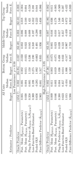
Table 2: Mon te Carlo Exp erimen t 1: Random Eects, Parametric Tw eed ie Correction, Selection Bias All Units Bottom Group Mid dle Group Top Group Median Median Medi an Median Estimator / Predictor Regret Forec.E. Regret Forec.E. Regret Forec.E Regret Forec.E. Lo w Persistence: ρ = 0 . 50 Oracle Predictor (12 52.7) 0.002 (65.95) -0.037 (62.48) 0.003 (62.10) -0.003 Post. Mean (

ˆθQM

LE ,P arametric) 0.005 0.005 0.002 -0 .0 30 0.002 0.006 0.018 -0.004 Post. Mean (

ˆθGM

M ,P arametric) 0.030 0.004 0.015 -0.035 0.022 0.008 0.100 0.004 Plug-In Predictor (

ˆθGM

M

,

ˆλ(i

ˆθGM

M ) ) 0.358 0.005 1.150 0.536 0.045 0.009 1.421 -0 .5 58 Loss-F unction-Based Estimator 0.369 0.199 0.275 0.190 0.348 0.197 0.352 0.188 Po oled OLS 0.656 -0.285 1.892 -0 .6 63 0.491 -0.288 0.223 0.044 First-Dierence Predictor (

ˆθGM

M ) 2.96 3 0.001 5.317 0.935 1.936 0.009 5.656 -0.986 High Persistence: ρ = 0 . 95 Oracle Predictor (12 52.7) 0.002 (67.36) -0.081 (63.16) 0.007 (61.86) -0.002 Post. Mean (

ˆθQM

LE ,P arametric) 0.009 0.011 0.003 -0 .0 75 0.005 0.016 0.036 0.015 Post. Mean (

ˆθGM

M ,P arametric) 0.046 0.003 0.019 -0.071 0.023 0.010 0.178 -0.005 Plug-In Predictor (

ˆθGM

M

,

ˆλ(i

ˆθGM

M ) ) 0.380 0.004 1.036 0.498 0.039 0.017 1.546 -0 .5 69 Loss-F unction-Based Estimator 0.623 0.357 0.014 0.033 0.522 0.357 1.358 0.597 Po oled OLS 1.015 -0.454 1.066 -0 .5 17 0.967 -0.459 0.872 -0.422 First-Dierence Predictor (

ˆθGM