University of Pennsylvania
ScholarlyCommons
Publicly Accessible Penn Dissertations
2017
Balancing Multiple Goals In Observational Study
Design
Samuel Pimentel
University of Pennsylvania, [email protected]
Follow this and additional works at:https://repository.upenn.edu/edissertations
Part of theStatistics and Probability Commons
This paper is posted at ScholarlyCommons.https://repository.upenn.edu/edissertations/2530
For more information, please [email protected].
Recommended Citation
Pimentel, Samuel, "Balancing Multiple Goals In Observational Study Design" (2017).Publicly Accessible Penn Dissertations. 2530.
Balancing Multiple Goals In Observational Study Design
Abstract
This thesis unites three papers discussing new strategies for matched pair designs using observational data, developed to balance the demands of various disparate design goals. The first chapter introduces a new matching algorithm for large-scale treated-control comparisons when many categorical covariates are present. The algorithm balances covariates and their interactions in a prioritized manner by solving a combinatorial optimization problem, and guarantees computational efficiency through the use of a sparse network representation. The second chapter defines a class of variables called prods which can be ignored when matching in order to strictly attenuate unmeasured bias, if it is present. These variables can be difficult to identify with confidence, so a multiple-control-group strategy is proposed in which investigators match once on all variables, and once ignoring prods; the two treated-control comparisons together give stronger evidence about treatment effects than either one individually. The final paper considers a new version of Fisher's classical lack-of-fit test for regression models, appropriate for data that lack replicated observations. The test uses matched pairs formed by optimal nonbipartite matching as near-replicates, and the model fit is used is used in constructing the matching distance in order to focus attention on variables that are predictive in the null model.
Degree Type
Dissertation
Degree Name
Doctor of Philosophy (PhD)
Graduate Group
Statistics
First Advisor
Paul Rosenbaum
Keywords
Causal Inference, Combinatorial optimization, Lack of fit, Matching, Network flow optimization, Unmeasured bias
Subject Categories
BALANCING MULTIPLE GOALS IN OBSERVATIONAL STUDY DESIGN
Samuel D. Pimentel
A DISSERTATION
in
Statistics
For the Graduate Group in
Managerial Science and Applied Economics
Presented to the Faculties of the University of Pennsylvania
in
Partial Fulfillment of the Requirements for the
Degree of Doctor of Philosophy
2017
Supervisor of Dissertation
Paul Rosenbaum, Robert G. Putzel Professor; Professor of Statistics
Graduate Group Chairperson
Catherine Schrand, Celia Z. Moh Professor; Professor of Accounting
Dissertation Committee:
Dylan Small, Class of 1965 Wharton Professor of Statistics
Jeffrey Silber, Nancy Abramson Wolfson Endowed Chair in Health Ser-vices Research, Children’s Hospital of Philadelphia; Professor of Health Care Management
BALANCING MULTIPLE GOALS IN OBSERVATIONAL STUDY DESIGN
COPYRIGHT
2017
Acknowledgments
I would like to thank my advisor Paul Rosenbaum for his substantial involvement
and influence in every stage of my development as a student and scholar. Besides
introducing me to a wide range of interesting research problems and helping me
week-by-week to break them into smaller, achievable tasks, Paul showed incredible patience
through the dry periods of my research, gave heartening encouragement and praise
at every step, and immediately provided wise and thoughtful advice on any aspect
of my academic life whenever I asked. Paul’s perspective and example has been and
will surely continuing to be a guiding light in all my academic thought and writing.
Dylan Small also spent countless hours with me during my Ph.D., both as an
instructor in foundational courses that underpinned my later research and as an
advisor and co-author in more recent years. His creative insights on challenging
research problems and his tremendous example of effective collaborative work have
been an inspiration.
I am also indebted to the other members of my dissertation committee. Jeffrey
Silber introuduced me to rich datasets and compelling questions in modern medical
research, for willingly became an early adopter of my statistical software, and boosted
Krieger provided a patient listening ear and an illuminating perspective on my work
as it developed, and he also imparted invaluable support and advice as I prepared for
and went on the job market.
I was fortunate to work with several other supportive collaborators — notably
Rachel Kelz, Luke Keele, and Guy Grossman — who introduced me to new areas of
application for my methods, invested many hours in our joint projects, and helped me
develop confidence as an independent collaborator. The members of the Center for
Causal Inference at Penn also provided a stimulating intellectual community, helping
me workshop my own ideas and bringing me up to speed on important work across
our field.
The NDSEG program of the Department of Defense and the Penn Family Grant
program both provided me with generous funding during my Ph.D., and I greatly
appreciate the support of those programs and their staff.
Maggie Saia and Gidget Murray of Wharton Doctoral Programs cheerfully guided
me through the administrative process of obtaining my degree and provided me with
many fulfilling opportunities to give service to the University outside of my
depart-ment.
I owe much to the faculty of the Statistics Department, particularly Mark Low,
Mike Steele, Ed George, Larry Brown, Linda Zhao, and Andreas Buja, and to its
staff, particularly Adam Greenberg, Noelle Felipe, Carol Reich, Sarin Sieng, and
Tanya Winder. All made themselves approachable from my first day at Penn and
provided much-needed advice and support in diverse aspects of my life as a graduate
student.
I am also very grateful for the friendship of my fellow graduate students in the
Statistics Department during our shared journey. My cohort-mates Zijian Guo,
pro-vided a wonderful community, both rejoicing in my successes with me and helping
me work through more challenging times. Several former students of the department
have also played key roles as mentors to me, including Jose Zubizarreta, Frank Yoon,
Mike Baiocchi, and Adam Kapelner.
Finally, I am very grateful for the love and support of my immediate and extended
family. Above all, my wife Maren and my sons Caleb and Jeremy have been my biggest
supporters, and have demonstrated the highest levels of patience and personal sacrifice
ABSTRACT
BALANCING MULTIPLE GOALS IN
OBSERVATIONAL STUDY DESIGN
Samuel D. Pimentel
Paul Rosenbaum
This thesis unites three papers discussing new strategies for matched pair designs
us-ing observational data, developed to balance the demands of various disparate design
goals. The first chapter introduces a new matching algorithm for large-scale
treated-control comparisons when many categorical covariates are present. The algorithm
balances covariates and their interactions in a prioritized manner by solving a
combi-natorial optimization problem, and guarantees computational efficiency through the
use of a sparse network representation. The second chapter defines a class of
vari-ables called prods which can be ignored when matching in order to strictly attenuate
unmeasured bias, if it is present. These variables can be difficult to identify with
con-fidence, so a multiple-control-group strategy is proposed in which investigators match
once on all variables, and once ignoring prods; the two treated-control comparisons
together give stronger evidence about treatment effects than either one individually.
The final paper considers a new version of Fisher’s classical lack-of-fit test for
uses matched pairs formed by optimal nonbipartite matching as near-replicates, and
the model fit is used is used in constructing the matching distance in order to focus
Contents
1 Introduction 1
2 Large, Sparse Optimal Matching with Refined Covariate Balance 4
2.1 Introduction . . . 4
2.2 Abstract problem . . . 7
2.3 Patient outcomes achieved by new and experienced surgeons . . . 10
2.4 A network algorithm . . . 17
2.5 Do new and experienced surgeons differ? . . . 29
2.6 Discussion of other applications of the methodology . . . 34
3 Constructed Second Control Groups and Attenuation of Unmea-sured Biases 36 3.1 Introduction: background; motivating example . . . 36
3.2 Review of notation and definitions . . . 39
3.3 When does ignoring an observed covariate produce attenuation? . . . 43
3.4 The magnitude of the attenuation . . . 49
3.5 Two control groups: controlling for (x, xe) or x . . . 50
3.7 Summary: Prefer additional analyses to additional assumptions . . . 64
4 An Exact Test of Fit for the Gaussian Linear Model using Optimal Nonbipartite Matching 65 4.1 Notation and review . . . 65
4.2 An exact test of fit for the Gaussian linear model . . . 69
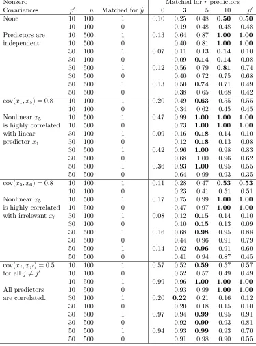
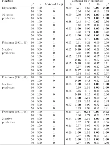
4.3 Simulation study of the power of the test . . . 73
4.4 Example: testing fit without replicates in an experiment . . . 79
4.5 Discussion: Summary; Alternative methods for selecting variables . . 81
5 Conclusion 85 A Appendices 89 A.1 Proofs of main results in Chapter 2 . . . 89
A.2 Formal description of matching algorithm in Chapter 3 . . . 93
List of Tables
2.1 Refined balance on six nominal variables in new surgeons study . . . 14
2.2 Covariate imbalance before and after matching . . . 16
2.3 Mortality results . . . 32
2.4 Sensitivity analysis for mortality results . . . 33
3.1 Bias attenuation from ignoring a prod . . . 54
3.2 Bias attenuation from separating groups on a prod . . . 54
3.3 Standardized differences on the prod after matching with separation . 54 3.4 Sensitivity analysis in example with two control groups . . . 61
3.5 Simulated power of sensitivity analysis with two control groups . . . . 63
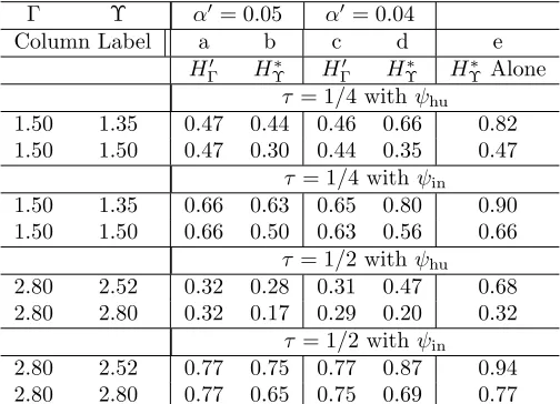
4.1 Simulated power of test for a nonlinear data-generating model under different design distributions . . . 76
List of Figures
1
Introduction
This thesis is based on three papers, all of which address the need to balance several
possibly disparate goals in forming matched pair designs using observational data.
The first paper considers a large-scale comparison of the health outcomes of patients
treated by new surgeons and those of patients treated by experienced surgeons, using
data from Medicare claims. Matching new surgeon patients to similar experienced
surgeon patients in this observational study provides a special analytic and
computa-tional challenge, because of the volume of data but also because of the large number
of complex categorical covariates measured for the patients. A new network flow
algorithm is presented for matching in this setting, incorporating novel balancing
constraints that remove pre-treatment group differences on categorical covariates and
their interactions in order of scientific priority. Furthermore, the algorithm represents
large observational studies as sparse network flow problem, allowing matches of
un-precedented size to be constructed efficiently. In the surgical study, the algorithm
produced very desirable levels of balance on interactions of many nominal covariates.
This project is joint work with Rachel Kelz, Jeffrey Silber, and Paul Rosenbaum, and
was published in 2015 in Volume 110, Issue 510 of the Journal of the American
Sta-tistical Association. It was produced with support by Grant SBS 1260782 from the
National Institute of Aging, and by Fellowship FA9550-11-C-0028 from the
Depart-ment of Defense, Army Research Office, National Defense Science and Engineering
Graduate (NDSEG) Fellowship Program, 32 CFR 168a4.
The second paper addresses an important question, frequently arising in practice,
about which variables to use for matching in observational studies. Randomized
tri-als balance all covariates, observed and unobserved; matching analyses generally try
to balance all observed covariates (since it cannot directly balance unobserved
co-variates). However, informal arguments in the applied medical literature claim that
matched analyses would admit less bias due to unobserved covariates if certain
ob-served variables were left unbalanced. This work formalizes that argument and prove
that a certain class of variables, called “prods” to receive treatment, can be left
un-balanced in the match to strictly lower the degree of unmeasured bias. In practice
it is difficult to identify these variables, since they are defined by uncheckable
condi-tions. It is suggested the result is most useful in the computerized construction of a
second control group, where the investigator can see more in available data without
necessarily believing the required conditions. One of the two control groups controls
for the possibly irrelevant observed covariate, the other control group either leaves
it uncontrolled or forces separation; therefore, the investigator views one situation
from two angles under different assumptions. A pair of sensitivity analyses for the
two control groups is coordinated by a weighted Holm or recycling procedure built
around the possibility of slight attenuation of bias in one control group. Issues are
illustrated using an observational study of the possible effects of cigarette smoking
as a cause of increased homocysteine levels, a risk factor for cardiovascular disease.
This is joint work with Dylan Small and Paul Rosenbaum, and was published in 2015
in Volume 111, Issue 515 of the Journal of the American Statistical Association. It
Pro-gram of the National Science Foundation and by Fellowship FA9550-11-C-0028 from
the Department of Defense, Army Research Office, National Defense Science and
Engineering Graduate (NDSEG) Fellowship Program, 32 CFR 168a4.
The final paper considers an alternative use of matching, not for formation of
comparison groups in an observational study but for use in testing the fit of a linear
regression model. Fisher’s classical lack-of-fit test uses perfectly replicated
obser-vations to produce a second estimate of the model standard error and conduct a
goodness-of-fit test, but in practice observational datasets rarely contain perfectly
replicated observations. A new test is presented, which identifies near-replicates for
use in Fisher’s testing framework via optimal nonbipartite matching. In particular,
a distance is defined for use in the matching algorithm that focuses on predictors
important in the original model, betting that model failures involve variables
impor-tant in the original fit. The test is shown to be exact, despite its use of the original
fitted model, and to have reasonable power even when the true set of predictors is
hidden within a large collection of spurious ones. This is joint work with Dylan Small
and Paul Rosenbaum, and is forthcoming inTechnometrics, and was conducted with
support by National Science Foundation Grant SES-1260782 from the Measurement,
Methodology and Statistics Program of the NSF and by Fellowship FA9550-11-C-0028
from the Department of Defense, Army Research Office, National Defense Science and
2
Large, Sparse Optimal Matching with Refined
Covariate Balance
2.1
Introduction: Matching within natural blocks
2.1.1
What are natural blocks?
In observational studies of treatment effects, we often wish to compare treated and
control subjects from the same natural block. Familiar examples of natural blocks are
twins, siblings, surgical patients in the same hospital, or students in the same school.
Important unmeasured covariates may be more similar within a natural block than
between blocks: the genes of siblings; the nursing staff and intensive care unit in
the same hospital; the teaching staff and socioeconomic conditions within the same
school.
There can be a tension between the desire to compare treated and control
individ-uals within natural blocks and the desire to compare treated and control groups with
similar distributions of measured covariates. In our study in§3.1 comparing new and
experienced surgeons, there are 1252 natural blocks of a new and experienced
sur-geon performing similar types of surgery working in the same hospital. Additionally
ultimately nearly 2.9 million categories defined by measured covariates. With many
categories, it is difficult if not impossible to find similar patients inside the same
natural block.
Attempts to balance many covariates by pairing individuals who are nearly
iden-tical almost invariably fail because nearly ideniden-tical people do not exist. This is
illustrated in Zubizarreta et al. (2011, Table 6; 2014, §2.4) where close individual
pairs are not available but covariate balance is attainable. Matching for a scalar
propensity score can balance many covariates such as age or gender, but this
ap-proach can perform poorly with sparse nominal covariates having many categories,
for instance the 176 surgical procedures and their interactions with comorbidities.
Like randomization, matching on propensity scores balances covariates stochastically
with the aid of the law of large numbers, whereas a nominal covariate with many
categories may have small sample sizes in most categories.
Our algorithm pairs patients within a natural block, trying to pick individual pairs
that are close on covariates. There is a limit to what can be achieved by finding
individually close pairs on many variables, so a separate effort is made to balance
distributions of covariates when individuals within a pair may differ. The approach
comes as close as possible to balance for a sequence of nested nominal variables,
starting with the 176 surgical procedures, gradually subdividing these 176 categories
to finally reach nearly 2.9 million categories involving comorbidities and admission
source, obtaining the best possible balance at each successive stage of the subdivision.
This new objective, “refined covariate balance,” is defined in§2.4.4, where it is proved
in Theorem 6 that our new network optimization algorithm yields a minimum distance
match subject to the constraint of refined covariate balance. This new approach is
2.1.2
Natural blocks and network sparsity
Optimal matching in observational studies (Rosenbaum, 1989; Hansen, 2007) is often
implemented using network optimization, a collection of mathematical and
compu-tational techniques originally developed to solve problems in operations research; see
the review of network optimization in §2.4.3. A network is a set of nodes together
with a set of directed edges or ordered pairs of nodes. Think of the nodes as subjects
and the edges as candidate pairings of two subjects. A network withN nodes might
haveN2 edges with loops or N(N−1) edges if with no loops; that is, it might have
O(N2) edges asN → ∞and in this case the network is said to be dense. A network
is said to be sparse if the number of edges is O(N) rather than O(N2). Matching
within natural blocks, such as within hospital-surgeon-pairs, drastically restricts the
number of permitted pairings of patients, resulting in a sparse network. The time
and space required for optimization is much greater in dense than in sparse networks
(e.g., Korte and Vygen 2008, Theorem 9.17).
Typical uses of optimal matching in observational studies do not exploit sparsity,
in part because a network defined by measured covariates without natural blocks is
likely to be dense. A program such as Hansen’s (2007) optmatch package in R can match thousands of individuals at once in a dense network. In current practice,
if a problem has many more than thousands of individuals, then it is divided into
smaller problems each consisting of thousands of individuals by matching exactly for
several important covariates. This strategy often works well for measured covariates.
However, with natural blocks, there may be relatively few choices within blocks, so
more of the work needs to be done through balancing covariate distributions. By
working with a network that is naturally sparse because of natural blocks, we are able
to match hundreds of thousands of individuals at once, thereby making much more
2.1.3
Outline: an example; a new objective; a new algorithm;
the benefits of sparsity
The surgical example is discussed in§3.1 and§2.5. The general problem is described
informally in §2.2 and developed precisely in §2.4. All new results and methods
are contained in §2.4. Notation is introduced in §2.4.1, key concepts such as refined
balance are defined in§2.4.2, and existing literature on network optimization is briefly
reviewed in §2.4.3. The matching network for refined balance is defined in §2.4.4.
The main theorem in §2.4.5 says that a minimum cost flow in the network defined in
§2.4.4 is the closest possible match that exhibits refined balance while respecting the
natural blocks. Sparsity is discussed in§2.4.7. The discussion in §2.6 considers how
the proposed methods might be applied in other contexts.
For discussion of matching, see Baiocchi et al. (2012), Hansen and Klopfer (2006);
Hansen (2007), Heller et al. (2009), Lu et al. (2011), Rosenbaum (1989, 2010),
Rosen-baum and Rubin (1985), Stuart (2010), Yang et al. (2012), and Zubizarreta et al.
(2011, 2014). For recent applications of optimal matching, see Silber et al. (2013)
and Neuman et al. (2014).
2.2
Abstract problem; intuition behind its
solu-tion; other applications
2.2.1
The abstract problem: refined balance in a sparse match
In a sparse matching problem, each treated subject has a short list of potential
con-trols. When there are natural blocks, this short list consists of controls from the
same block; however, sparse networks arise or can be produced in other ways; see
each given treated subject does not increase. As you add more and more families
or schools or hospitals or zip codes to the study, you have more and more subjects
to match, but individual families or schools or hospitals or zip codes do not become
larger. If the number of blocks increases in constant proportion to the increase in
total sample size, then block effects are not consistently estimable without
assump-tions about their form (Kiefer and Wolfowitz, 1956, p. 888); however, it is possible
to match within blocks.
In addition to picking for each treated subject a control from the short list of
candidates, the matching must balance many observed covariates. We would be
satisfied if the balance on observed covariates after matching were similar to the
balance on observed covariates in a completely randomized experiment, but this may
not be possible in an observational study. Randomization also balances unmeasured
covariates whereas matching for observed covariates cannot be expected to do this.
Because the list of candidate controls for a given treated subject is short, it is rarely
possible to find a control on the short list who is identical to the treated subject with
respect to many covariates. So the matching algorithm tolerates a mismatch in one
pair providing it can counterbalance that mismatch in another pair. If it is necessary
to match a treated male to a control female in one block, then a treated female will be
matched to a control male in another block, so the final treated and control groups
have exactly the same number of males and the same number of females. Exact
counterbalancing is called “fine balance”; see Rosenbaum et al. (2007). Fine balance
means that the marginal distribution of a categorical covariate is exactly the same in
treated and control groups, and in the surgical example the 176 surgical procedures are
finely balanced. Counterbalancing is a familiar strategy in experimental design, for
example in Latin square designs or crossover designs. Sometimes exact fine balance
balance all 2.9 million categories of patients. “Near fine balance” means that the
marginal distributions of a categorical covariate in matched samples are “as close as
possible” to fine balance given the data available; see Yang et al. (2012). In defining
near fine balance, one may define “as close as possible” in various ways, but one
natural and familiar measure is the total variation distance, the sum of the absolute
treated-minus-control differences in category percents. See Arratia et al. (1990, §3)
for several attractive equivalent definitions of the total variation distance. If the
matched treated group is 51% male and the matched control group is 49% male, then
the total variation distance in gender is |0.51−0.49|+|0.49−0.51|= 0.04 reflecting
the 2% mismatch for males plus the corresponding 2% mismatch for females. One
form of near fine matching minimizes the total variation distance in matched samples,
and it achieves exact fine balance whenever this is achievable.
Refined balance is an extension of fine or near-fine balance. One defines a sequence
of nested nominal variables,ν1, . . . ,νK, soνk+1subdividesνk. Refined balance comes
as close as possible to fine balance forν1, and among all matches that do that, it comes
as close as possible to fine balance for ν2, and so on. In the surgical example, ν1
consists of the 176 surgical procedures and these are finely balanced, ν2 interacts the
176 surgical procedures with two types of hospital to make 352 categories for which
the minimum total variation distance is 0.001 or one tenth of 1%, . . . , and vK for
K = 6 has 2.9 million categories. Among all matched samples that exhibit refined
covariate balance, the algorithm finds pairings from the short lists to minimize the
total covariate distance within pairs.
2.2.2
Intuition behind the solution
In §2.4, the matching problem is represented by a network or directed graph. For
to a match. One route is free of charge, and a pair can take this route if it leaves this
category balanced. The other route has a large toll or penalty, and a pair can take this
route without balancing the category but must pay the penalty. The penalty forν1 is
much larger than for ν2, and so on. The objective function is the sum of all of these
penalties plus the sum of the within-pair covariate distances. The penalization of
certain paths is developed in detail in §2.4.4 and it involves a parameter Υ. Network
optimization minimizes this penalized objective function. If the penalties are both
sufficiently large and sufficiently different forνk andνk+1, then they override all other
considerations, producing refined balance. Among all matches that minimize the
penalties, the optimal match minimizes the sum of the covariate distances. In the
example, among matches that are equally good in terms of refined covariate balance,
the algorithm tried to pair individuals with similar ages and estimated risks of death,
two variables that were not explicitly balanced. Section 2.4 states the algorithm
precisely and proves that it works.
Refined balance and sparsity are separate ideas that work well together. In a
sparse network, it is difficult to find close individual pairs, and more of the work must
be done by covariate balancing; hence, the attraction of refined balance for sparse
problems. Conversely, balancing of rare categories is easier in very large problems,
and computations for large problems require less computer time and storage if the
problem is sparse; hence the attraction of sparsity for refined balance. Sparsity is
2.3
Patient outcomes achieved by new and
expe-rienced surgeons
2.3.1
Background
Are the patient outcomes of newly trained surgeons comparable to the outcomes of
experienced surgeons performing the same types of surgery at the same hospitals? If
the typical patient of the typical new surgeon were instead treated by an experienced
surgeon, would the patient’s outcomes be different? The data describe patients in
Medicare in six states between 2004 and 2007 who had Medicare Part B, were not in
a Medicare HMO, and had surgery performed at a hospital rather than on an
out-patient basis at an ambulatory surgical center. Here, we look at 6260 out-patients of 1252
new surgeons and 6260 patients of 1252 experienced surgeons at the same hospitals,
5 patients per surgeon.
Surgical skill varies from surgeon to surgeon. Are the worst surgeons also the
new surgeons? A typical hospital might have one new surgeon and a group of
experi-enced surgeons. We expect that the performance of individual new surgeons will be
more variable, more extreme, than the average performance of a group of experienced
surgeons, simply because averages are more stable than individuals. Surgeons
special-ize, focusing on particular types of surgery, and the 30-day mortality rate following,
say, elective orthopedic surgery is much lower than for some types of cancer surgery.
These considerations, together with desire for a simple, transparent study design, led
us to pair each new surgeon with an experienced surgeon performing similar types of
surgery at the same hospital.
New surgeons gradually become experienced surgeons. As they become more
experienced, they perform more surgery. Most of the population of patients of new
interested in new surgeons when they are starting out, when most of their experience
is from surgical training. For these reasons, we decided to give equal weight to each
young surgeon, rather than weighting surgeons by the number of operations they
performed. We considered only new and experienced surgeons who had performed
at least five operations in our data. We sampled at random five surgical patients of
each new surgeon as the treated group. For many newer new surgeons, five patients
was a large part of the portion of the overlap of their surgical practice with our
data. Our analysis describes the typical patient of the typical new surgeon, not the
typical patient of new surgeons as a group, the latter being weighted towards the
most experienced new surgeons.
2.3.2
Matching the patients of new and experienced surgeons
within the same hospital
Surgical data are characterized by quite a bit of detail, much of it recorded in
nom-inal variables. Using ICD-9 codes, we distinguish 176 surgical procedures (listed in
Table 2.1 as Procedure). In addition, we distinguish among 498 hospitals, whose
per-formance varies for reasons unrelated to surgical perper-formance. Patients often have
existing medical problems, called comorbidities, besides those treated by the current
surgery, such as congestive heart failure (CHF) or chronic obstructive pulmonary
disease (COPD), and these may increase the risk of death following surgery. We
distinguish hospitals with many new surgeons or few new surgeons (Hospital Group).
Patients are matched within surgeon pairs within the same hospital.
Table 2.1 lists covariates that structure the match, and additional covariates
ap-pear in Table 2.2. Table 2.1 includes notation that will be defined in §2.4. In
the rows of Table 2.1, there are 15 nominal covariates, making 176×214 or about
covariates, ν1, . . . , ν6, where ν1 is simply the L1 = 176 procedures, ν2 is the 176
procedures crossed with Hospital Group with L2 = 176×2 = 352 categories, ν3 is
the 176 procedures crossed with Hospital Group, male, ER-admission, and
Transfer-admission with L3 = 176×24 = 2816 categories, . . . , and ν6 crosses all 15 covariates
with 176×214= 2. .9 million categories.
Ideally, the number of patients of new surgeons in each of 2.9 million categories
would equal the number of patients of experienced surgeons. That was not quite
possible while always also matching patients within the 498 hospitals. Subject to
that requirement of matching within hospitals, the match minimized imbalance in a
sense to be defined in a moment, and minimized the sum of a covariate distance over
6260 patient pairs.
A nominal covariate with Lk levels yields an Lk×2 contingency table with two
columns for the patients of new and experienced surgeons. In the matched sample,
each column contains a total of 6260 patients distributed among Lk categories or
rows. How different are the distributions in the two columns? Write βk` for the
difference in counts of νk in row ` of the table; then 0 = PL`=1k βk` and PL`=1k |βk`| is
proportional to a standard measure of the difference between two discrete probability
distributions, namely the total variation distance. Now, PLk
`=1|βk`| could be as small as 0 if the distributions were identical or as large as 2×6260 = 12520 if they do not
overlap. To equalize the two distributions, one would need to switch the categories
for PLk
`=1|βk`|/2 controls or the percentage (100/6260)
PLk
`=1|βk`|/2.
The lower portion of Table 2.1 shows the total imbalance in the six nominal
covariates, ν1, . . . , ν6. For procedures, ν1, the imbalance was 0, so the distribution
of the 176 procedures is identical in the new and experienced groups. The imbalance
for ν1 is as small as possible. For ν2, the imbalance was 6, meaning that there was
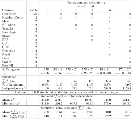
Table 2.1: The K = 6 nominal variables νk that were balanced as closely as possible by the matching algorithm, where ν1 consists of L1 = 176 surgical procedures, and ν6 is the
interaction of 176 surgical procedures with 14 binary covariates, making L6 = 176×211
categories, or about 2.9 million categories. An×indicates that the row variable contributes to nominal variable νk. The algorithm minimized the total imbalance
PLk0
`=1|βk0`| for νk0
among all matches that minimized PLk
`=1|βk`| for νk for k < k
0. The balance obtained by
matching is much better than the best balance obtained in 10,000 simulated randomized experiments with the same marginal totals.
Nested nominal covariate,νk
k= 1, . . . ,6
Covariate Levels 1 2 3 4 5 6
Procedure 176 × × × × × ×
Hospital Group 2 × × × × ×
Male 2 × × × ×
ER-admit 2 × × × ×
Transfer 2 × × × ×
Paraplegia 2 × × ×
Stroke 2 × × ×
PPF 2 × × ×
CC 2 × ×
CHF 2 × ×
Dementia 2 × ×
Renal 2 × ×
Liver 2 ×
Past A 2 ×
Past MI 2 ×
# Categories 176 176×2 176×24 176×27 176×211 176×214
Lk = 176 = 352 = 2,816 = 22,528 = 360,448 = 2,883,584 Imbalance
PLk
`=1|βk`| 0 12 52 176 664 1242
% of maximum 0.0% 0.1% 0.4% 1.4% 5.3% 9.9% Independenceχ2 0.0 4.9 43.3 142.3 588.9 1158.7
Balance in 10,000 simulated randomized experiments with the same margins Simulatedχ2 statistics for independence
Meanχ2 174.9 302.9 767.5 1062.0 1946.0 2814.0
Minimumχ2 117.0 226.5 645.7 933.6 1777.0 2645.0
Simulated Total ImbalancePLk
`=1|βk`|
MeanPLk
`=1|βk`| 768 1051 1749 2086 3010 3812
Min. PLk
in some other rows. The imbalance for ν2 is as small as possible among matches
that minimize the imbalance inν1. And so on. For ν6, the total absolute imbalance
is 1242 for 2 ×6260 = 12520 patients in 2.9 million categories, or about 10% of
the maximum imbalance. The imbalance for ν6 is as small as possible subject to
minimizing the imbalance in ν1, . . . , ν5 and matching within surgeon pairs. In
addition to producing a small imbalance inν1, . . . ,ν6, the matching algorithm certifies
that the imbalance attained is the smallest possible imbalance when matching new
and experienced surgeon patients within the same hospital; that is, there is no point
in trying to achieve a smaller imbalance.
The balance described in the previous paragraph is much better than
randomiza-tion would produce. We computed the usual χ2-statistic for independence in each
of the six 2×Lk contingency tables. We created 10,000 simulated randomized
ex-periments by simple random sampling without replacement of 6260 patients from the
12520 patients, so row and column margins of the 2×Lk are unchanged, and
com-puted 10,000 independence χ2-statistics and imbalances PLk
`=1|βk`|; see the bottom of Table 2.1. For ν6 with 2.9 million categories, the actual matched sample had an
imbalance of 1242 andχ2 of 1158.7, and that was much better balance than the best
of 10,000 simulated randomized experiments with an imbalance of 3578 and χ2 of
2645.0.
Subject to the constraints of matching within hospital and minimizing imbalance
PLk
`=1|βk`| in Table 2.1, the algorithm minimized the total over 6260 patient pairs of
a covariate distance within pairs. Table 2.2 looks at the imbalance on the individual
matching variables, including age and the risk score, neither of which is in Table 2.1.
Do new surgeons treat the easiest patients? Apparently not. In Table 2.2, before
matching, the patients of new surgeons are much more likely to have entered through
Table 2.2: Covariate imbalance before and after matching. The table compares new surgeons to experienced surgeons, before and after matching, in term of covariate means, standardized differences in means as a fraction of the standard deviation before matching, and two-sampleP-values. New = new surgeon, Ex-B = experienced surgeon, before matching, Ex-A = experienced surgeon, after matching. Standardized differences above 1/10th of a standard deviation are in bold.
Covariate Mean Standardized Difference 2-sample P-value Covariate New Ex-B Ex-A Before After Before After Sample size 6,260 123,846 6,260
are more likely to have dementia, and tend to be older. These differences are largely
absent after matching. New surgeons are treating a challenging and vulnerable group
of patients. In §2.5, we ask: How do outcomes compare for new and experienced
surgeons when experienced surgeons treat equally challenging patients?
2.4
A network algorithm for large, sparse optimal
matching with refined balance
2.4.1
Notation: acceptable 1-to-
m
match; covariate
imbal-ance
β
k`There are T treated subjects, T = {τ1, . . . , τT}, and C ≥ T potential controls, C =
{κ1, . . . , κC}, with ∅ = T ∩ C. In §2.3.2, T contains patients of new surgeons and
C contains patients of experienced surgeons. Write |S| for the number of elements
in a finite set S, so that T = |T |. There were T = 6260 patients of new surgeons
to be matched and C = 123846 candidate control patients of experienced surgeons.
Treated subject τt ∈ T has observed covariate xτ t and potential control κc ∈ C has
covariate xκc.
There is a subset of acceptable pairings, A ⊆ T × C, such that (τt, κc) is an
acceptable pairing if and only if (τt, κc) ∈ A. In §2.3.2, we had previously paired a
new and an experienced surgeon at the same hospital performing similar procedures,
and the acceptable pairingsAare only of patients of these paired new and experienced
surgeons at the same hospital; that is, (τt, κc) ∈ A if and only if τt is a patient of
a new surgeon and κc is a patient of the experienced surgeon with whom this new
surgeon is paired. In§2.3.2, |A|= 819230 <7.75×108 =T ×C =|T × C|.
For each (τt, κc)∈ A there is a distance δtc betweenxτ tand xκc, δtc =δ(xτ t,xκc),
§2.3.2,δtc =δ(xτ t,xκc) was a robust, rank-based Mahalanobis distance (Rosenbaum,
2010, §8) based on age, sex, emergency admission, transfer admission, risk score and
clusters of procedures. There is competition for controls, so κc may be the closest
control to both τt and τt0, and an optimal matching will minimize the total distance
for matched individuals subject to various constraints on the balance of covariates.
There are K nested nominal variables νk(·), k = 1, . . . , K; that is, νk(·) is a
function that assigns one of Lk values in Kk = {λk1, . . . , λk,Lk} to each subject in
T ∪ C, or νk : T ∪ C → Kk. In §2.3.2 and Table 2.1, there were K = 6 nominal
variables. Importantly, νk+1 refines or subdivides νk. In other words, these K
variables are nested in the sense that all individuals who are the same on νk+1 are
the same on νk; that is, formally, if ι ∈ T ∪ C with νk+1(ι) = λk+1,` and ι0 ∈ T ∪ C
with νk+1(ι0) = λk+1,`, then νk(ι) = νk(ι0). Variable ν1(·) is the coarsest and most
important variable and νK(·) is the finest and least important variable. Expressed
informally, the algorithm will do everything possible to balance ν1(·) as closely as
possible, whereas it will merely do what it can to balance νK(·).
Definition 1 Acceptable 1-to-m match: An acceptable 1-to-m match is a subset
M ⊆ A such that every τt ∈ T appears in exactly m pairs (τt, κc) ∈ M and every
κc∈ C appears in at most one pair (τt, κc)∈ M.
If A = T × C, then an acceptable 1-to-m match exists whenever C ≥ mT. If
A ⊂ T ×C, then an 1-to-macceptable match may not exist even whenC ≥mT. The
algorithm finds an acceptable 1-to-mmatch if one exists; otherwise it reports that no
such match exists. The conditions required for the existence of an acceptable match
are stated in a famous theorem in graph theory, Hall’s theorem; see Diestel (2010,
Theorem 2.1.2, p. 38); however, the algorithm determines whether a match exists.
In addition to having an acceptable match withM ⊆ Awith a small total distance
P
over νk+1(·). Write dk` for the number of treated individuals τt falling in category
` of the kth nominal variable ν
k(·), so dk` = |{τt ∈ T :νk(τt) =λk`}|. Ideally, an
acceptable 1-to-m match Mwould havem×dk` matched controls falling in category
` of the kth nominal variableν
k(·), so the distributions of νk(·) would be identical in
matched treated and control groups; however, typically, this is not possible for larger
k. That is, ideally |{(τt, κc)∈ M:νk(κc) =λk`}| would equal m×dk` for every k
and `. Because the K variables are nested, an imbalance in νk(·) is necessarily also
an imbalance in νk+1(·).
The imbalance βk` in the `th category of the kth nominal variable is a signed
integer that is m times the number of treated subjects τt inM with level λk` of the
kth nominal variable minus the number of controls κ
c inM with level λk`, that is,
βk`=m×dk`− |{(τt, κc)∈ M :νk(κc) =λk`}|. (2.1)
In (2.1),βk` depends upon the matchMthrough |{(τt, κc)∈ M :νk(κc) = λk`}|, but
the notation does not indicate the dependence explicitly; that is, some matches M
exhibit better covariate balance than do others. Hereβk` >0 signifies that we wanted
more controls at level`of nominal variableνk(·), andβk` <0 signifies that we wanted
fewer. By the definition of an acceptable 1-to-m match, for each k, the total of the
signed imbalances is zero, 0 =PLk
`=1βk` (i.e., everyone has to go somewhere), but the total of the absolute imbalances PLk
`=1|βk`| measures the degree to which matched treated and control subjects have differing distributions of nominal variable νk(·).
In fact, (mT)−1PLk
`=1|βk`| is the total variation distance between the distribution of
νk(·) in matched treated and control groups. In Table 2.1,
PL3
`=1|β3`|= 52. In some
sense or other, we would like to pick an acceptable 1-to-m match such that each of
the PLk
`=1|βk`| is as small as possible and the within-pair distance
P
(τt,κc)∈Mδtc is as
The kth nested nominal variable is said to satisfy “fine balance” if β
k` = 0 for
` = 1, . . . , Lk, so νk(·) has the same distribution in matched treated and control
groups; see Rosenbaum et al. (2007). Because the K nominal variables are nested,
nominal variable νk(·) is finely balanced whenever νk+1(·) is finely balanced.
The kth nested nominal variable is said to satisfy “near fine balance” if matchM
minimizes PLk
`=1|βk`| among all acceptable 1-to-m matches; see Yang et al. (2012).
Because the K nominal variables are nested, PLk+1
`=1 |βk+1,`| ≥ PLk
`0=1|βk`0| for each k, as is seen in Table 2.1 where PL1
`=1|β1`| = 0≤ 12 = PL2
`=1|β2`| ≤ 52≤ . . .≤ 1242 = PL6
`=1|β6`|.
2.4.2
Two key definitions: What is an optimal refined
ac-ceptable 1-to-
m
match
M
?
Where fine and near fine balance refer to a single nominal variable, “refined balance”
refers to a nested sequence of nominal variables, such as νk(·), k = 1, . . . , K, as in
Table 2.1. Stated informally, each of thek levels is as balanced as possible, but level
k has priority over level k+ 1. Write Mfor the set of all acceptable 1-to-m matches
M. Each element M ∈ M is one possible match. Each such match M ∈ M
has values for βk` in (2.1) and a value for the total distance within matched sets,
P
(τt,κc)∈Mδtc. The two definitions that follow define a “best” choice of M ∈ M.
Definition 2 (Refined balance): An acceptable 1-to-m match M ∈ M has
re-fined balance if: (1) PL1
`=1|β1`| is minimized among all acceptable 1-to-m matches
M0 ∈ M , and (2) among acceptable 1-to-m matches that satisfy (1), M minimizes
PL2
`=1|β2`|, . . . , (k) among acceptable 1-to-m matches that satisfy (k-1), M mini-mizes PLk
`=1|βk`|, . . . , (K) among acceptable 1-to-m matches that satisfy (K-1), M minimizes PLK
For example, in Table 2.1, 52 is the minimum possible value of PL3
`=1|β3`| among all acceptable 1-to-1 matches with PL1
`=1|β1`|= 0 and PL2
`=1|β2`| ≤12.
Definition 3 (Optimal refined balance): An acceptable 1-to-m match M ∈
M with refined balance is optimal if it minimizes the total distance within pairs,
P
(τt,κc)∈Mδtc, among all acceptable 1-to-m matches M ∈M with refined balance.
The goal is to find an optimal refined acceptable 1-to-m match M if one exists
and otherwise determine that the problem is infeasible in that no such match exists.
2.4.3
Review of minimum cost flow in a network
The minimum cost flow problem is a standard combinatorial optimization problem
with origins in operations research; see Bertsekas (1991), Cook et al. (1998), and
Korte et al. (2008). This problem is a special type of integer program which, unlike
most integer programs, can be solved with a worst-case time bound that is a
poly-nomial in the size of the problem; that is, large problems can be solved quickly. A
standard way to “solve” a combinatorial optimization problem is to show that it is
equivalent to an appropriate minimum cost flow problem and to solve this equivalent
problem. (In R, a good solver for minimum cost flow problems can be obtained as follows. Hansen’soptmatchpackage calls Fortran codeRELAXIVcreated by Bertsekas et al. (1994) which solves minimum cost flow problems. Loading optmatch makes
RELAXIVaccessible inR and callable by imitating Hansen’s calls with different calling parameters. Documentation and code for RELAXIV are on Bertsekas’ web page at MIT.)
Metaphorically, objects are supplied and demanded at locations called nodes and
are shipped among nodes along edges connecting pairs of nodes, and the goal is to
Objects cannot be cut in half (e.g., TVs cannot be cut in half for shipping) so the
solution must ship integer rather than fractional objects. Companies like FedEx
solve minimum cost flow problems in a literal rather than metaphorical sense.
Op-timal matching problems are commonly reexpressed as minimum cost flow problems.
We find an optimal refined acceptable 1-to-m match M by solving an equivalent
minimum cost flow problem.
A network is a set of nodes, N, a set of edges E consisting of ordered pairs of
nodes, E ⊆ N × N, so each e ∈ E is of the form e = (n, n0) where n, n0 ∈ N. One
draws a network with a point for each node n ∈ N and an arrow connecting pairs of
nodes for which there is an edge e = (n, n0) ∈ E, where the tail of the arrow is at n
and the point of the arrow is at n0. See Figure 1, where the arrowheads are omitted
to limit clutter, but edges that are not horizontal point down and horizontal edges
point from right to left. Our network is acyclic or without cycles, so we may speak
of the early part of the network — the upper part in Figure 1 — or the late part of
the network — the lower part in Figure 1.
Each edge e ∈ E has a nonnegative, possibly infinite, integer capacity, cap(e) with 0≤cap(e)≤ ∞, and a nonnegative real cost, cost(e) with 0 ≤cost(e)<∞. That is, e can carry up to cap(e) units of flow and each unit costs cost(e) to transport over e. Each node n ∈ N has a finite integer demand, demand(n) with
−∞ < demand(n) < ∞. Node n absorbs demand(n) units of flow and passes the rest on, and demand(n)< 0 means n creates an excess of −demand(n) units of flow (e.g., manufactures −demand(n) TVs). A feasible flow f is a function that assigns a nonnegative integer f(e) to each edge e = (n, n0) ∈ E, such that: (i) the flow is
each node n∈ N is met,
X
n0:(n0,n)∈E
f{(n0, n)} − X
n00:(n,n00 )∈E
fnn, n00o=demand(n) for each n∈ N. (2.2)
The first sum in (2.2) is the total flow intonfrom neighboring nodesn0 with (n0, n)∈
E, while the second sum is the total flow out from n to neighboring nodes n00 with
n, n00 ∈ E, so the equation (2.2) says that node n absorbs demand(n) units of flow. A feasible flow may or may not exist. The total cost of a feasible flow is
P
e∈Ef(e) cost(e). An optimal feasible flow is any feasible flow that minimizes the
total cost. The problem of finding a minimum cost flow in a network has several fast
widely available solutions.
From a practical point of view, finding a minimum cost flow in a network may
be regarded by users as a standard mathematical computation, not unlike finding
the inverse of a matrix. The user specifies the network and is given a minimum
cost flow, as the user of matrix inversion software specifies a matrix and is given its
inverse. Not all matrices have inverses, and not all networks have feasible flows, and
in both cases competent software announces that the impossible has been requested.
A network is dense ifO(|E|) = |N |2.
2.4.4
The network for optimal refined acceptable 1-to-
m
matching
The network involves a penalization parameter, Υ > 1. Penalization will increase
the cost of a flow when that flow is behaving in a way we wish to avoid. In§2.4.5, it
will be shown that if Υ is large enough, then the solution to a certain minimum cost
flow problem yields an optimal refined acceptable 1-to-m matching.
Figure 2.1: A small network for refined covariate balance with treated subject
τ1, . . . , τ7, potential controls κ1, . . . , κ11, two balance layers λ1` and λ2`, and the sink
ω.
τ1 τ2 τ3 τ4 τ5 τ6 τ7
κ1 κ2 κ3 κ4 κ5 κ6 κ7 κ8 κ9 κ10 κ11
λ21 λ22 λ23
λ21’’ λ21’ λ22’’ λ22’ λ23’’ λ23’
λ11 λ12
λ11’’ λ11’ λ12’’ λ12’
the potential controls, C = {κ1, . . . , κC}, and an additional node ω called a sink.
Also the nodes contain all of the possible values of the K nested nominal variables,
Kk = {λk1, . . . , λk,Lk}, k = 1, . . . , K. Additionally, the nodes contain a primed
copy of values of the nested nominal variables, Kk0 =λ0k1, . . . , λ0k,L
k , k = 1, . . . , K,
and a double primed copy of all of the possible values of the nominal variables,
K00k = nλ 00
k1, . . . , λ 00
k,Lk
o
, k = 1, . . . , K. That is, the nodes are N = T ∪ C ∪ {ω} ∪
[K
k=1Kk∪ [K
k=1K 0
k∪
[K
k=1K 00
k.
If (τt, κc)∈ A ⊆ T × C is an acceptable pairing in the sense of§2.4.1, then (τt, κc)
is an edge of the network, (τt, κc) ∈ E with capacity cap{(τt, κc)} = 1 and cost
cost{(τt, κc)}=δtc, where δtc is the covariate distance betweenτtand κc introduced
in §2.4.1. There is an edge (κc, λK`) ∈ E connecting each potential control κc to
the category λK` of the last, most refined nominal variable νK(·) that contains this
control; moreover, this edge has capacity 1 and zero cost, cap{(κc, λK`)} = 1 and
cost{(κc, λK`)}= 0.
Every categoryk` of every nominal variableνk(·) appears as a small triangle inE
involving λk`, λ
0
k` and λ
00
k`. These triangles play an important role: each one makes
an effort to reduce a corresponding |βk`| in (2.1), recognizing that it may not be
possible to achieve |βk`| = 0. Every node λk` is connected to both λ
0
k` and λ
00
k`, so
λk`, λ
0
k`
∈ E and λk`, λ
00
k`
∈ E, and λ0k` is connected to λ 00
k` so
λ0k`, λ
00
k`
∈ E for
all k, `; that is, λk`, λ
0
k` and λ
00
k` form a triangle. There is, therefore, a direct path
from λk` to λ
00
k` and an indirect path from λk` to λ
00
k` that passes through λ
0
k`. As
discussed in §2.4.1, we would like to have m ×dk` controls in category λk` as this
would make βk` = 0 in (2.1); however, this may not be possible. The direct path
λk`, λ
00
k`
has cap
n λk`, λ
00
k`
o
= m×dk` and cost cost
n λk`, λ
00
k`
o
= 0, so that
up to m×dk` units of flow can move directly from λk` to λ
00
k` for free, without cost.
edge λk`, λ
0
k`
has infinite capacity, cap λk`, λ
0
k` = ∞, and severely penalized
cost ofcost λk`, λ
0
k` = ΥK
−k+1. The last leg of the triangle has infinite capacity
and zero cost, cap
n λ0k`, λ
00
k`
o
= ∞ and cost
n λ0k`, λ
00
k`
o
= 0. Notice that the
penalty for ν1(·) is ΥK but this gradually declines to penalty Υ for νK(·). Because
the coarse, most important ν1(·) is after the fine, less important νK(·), the penalties
in triangles increase from Υ for νK(·) to ΥK for ν1(·) as we move from start to the
end of the network. Informally, this says that a one-patient imbalance in vk(·) is
worse than a one-patient imbalance in vk+1(·).
The end λ00k` of a triangle at level k is connected to the beginning λk−1,`0 of the
coarser category k −1, `0 that contains category k`. This edge λ 00
k`, λk−1,`0
to a
coarsened category has infinite capacity and zero cost,cap
n λ
00
k`, λk−1,`0 o
=∞and
cost
n λ
00
k`, λk−1,`0 o
= 0. Finally, there is an edge fromλ 00
1` to the sink ωfor each `
with infinite capacity and zero cost, cap
n λ
00 1`, ω
o
=∞and cost
n λ
00 1`, ω
o
= 0.
For each τt ∈ T,demand(τt) = −m. The sink has demand(ω) = m|T |. All other
nodes have demand(n) = 0. In words, each treated node issues m units of flow, all nodes between the treated nodes and the sink pass on all the flow they receive, and
the sink ω collects all mT units of flow issued by the T treated units.
An important property of a feasible flow f in this network is that control node
κc ∈ C ⊂ N may receive either zero or one unit of flow, because 0 ≤ f(κc, λK`) ≤
cap{(κc, λK`)}= 1, and if f(κc, λK`) = 1 then there is only one possible sequence of
λ 00
k`’s along which that unit of flow can pass to the sink ω. For brevity, the network
defined in this section will be called “the network (N,E),” omitting explicit reference
2.4.5
Main result: A minimum cost flow yields an optimal
refined match
Lemma 4 says that the match we seek exists if and only if the minimum cost flow
problem is feasible. Proofs are in Appendix A.1.
Lemma 4 There is a feasible flow f for the network(N,E) if and only if there is an
acceptable 1-to-m match M. In particular, M={(τt, κc)∈ A:f{(τt, κc)}= 1}.
Lemma 5 relates total cost to matching quantities, namely total covariate distance
within pairs, P
(τt,κc)∈Mδtc, and the imbalance measuresβk` in (2.1).
Lemma 5 Suppose there is a feasible flow f in (N,E), let the associated match be
M={(τt, κc)∈ A:f{(τt, κc)}= 1}, and let βk` be the imbalance measure (2.1) for
match M. Then the cost of this flow satisfies
X
e∈E
f(e) cost(e)≥ X (τt,κc)∈M
δtc+ K
X
k=1
ΥK−k+1
Lk
X
`=1
|βk`|/2. (2.3)
If f is a minimum cost feasible flow in (N,E), then (2.3) holds as an equality.
Theorem 6 says we may find the match in Definition 3 by solving a standard
combinatorial optimization problem. There is a finite value (see§2.4.6) of the penalty
Υ such that for that value and for all larger values, the resulting match satisfies the
constraint of refined balance and minimizes the total covariate distance subject to
that constraint.
Theorem 6 If there exists a feasible flow in (N,E), then for sufficiently large Υ, a
minimum cost flow in (N,E) yields an optimal refined acceptable 1-to-m match M
given by M = {(τt, κc)∈ A:f{(τt, κc)}= 1}. If there exists no feasible flow in
2.4.6
Practical issues: deciding about
Υ
and
m
Theorem 6 speaks of “sufficiently large Υ,” and in its proof Υ is very large, specifically
Υ> mT K+P
(τt,κc)∈Aδtc. For stable computation, use a much smaller Υ, perhaps
Υ = 2 max(τt,κc)∈Mδtc or smaller. Theorem 6 says that as Υ increases, eventually the
imbalances PL1
`=1|β1`|, . . . , PLk
`=1|βk`| are the best possible imbalances and further increases in Υ do not change the imbalances, so it is reasonable to match a few times,
starting with a small Υ and gradually increasing it until the imbalances stop changing.
How many controls, m, should be matched to each treated unit? Match quality
decreases as m increases, so one might match m = 1 to 1, examine the resulting
average imbalances, (mT)−1PL1
`=1|β1`|, . . . , (mT)−1
PLk
`=1|βk`|, then matchm = 2 to
1, and so on, stopping when the quality of the match is not acceptable.
2.4.7
Computation in sparse networks
Algorithms are standardly evaluated in terms of an upper bound on the rate of growth
of the number of arithmetic steps required to solve them as the size of the problem
increases (Cook et al. 1998, §1.2; Korte et al. 2008, §1.2). If steps =O size3 then
the number of arithmetic steps required to solve a problem grows by at most a
con-stant multiple of the cube of the size of the problem. The point we want to make
in the current section is that: (i) the new surgeons problem, and more generally the
matching-within-natural-blocks problem, is sparse, with far fewer edges than
typi-cal matching problems, so (ii) vastly larger problems can be solved in these sparse
networks than can be solved in dense networks commonly appearing in statistical
matching problems, so (iii) we may balance covariates over an enormous number of
natural blocks.
The network (N,E) is dense if |E| = O |N |2
and sparse if |E| = O(|N |).
in O(|E|log [|E| {|E|+|N |log (|N |)}]) steps; see Korte and Vygen (2008, Theorem
9.17, p. 214). If |E| = |N |2, this is O
|N |2log (|N |) , whereas if |E| = |N | it is
O[|N |log{|N |}]. In §2.4.4, |N | > T +C = 130106 so |N |2log (|N |) is much larger
than |N |log (|N |).
2.5
Do new and experienced surgeons differ?
2.5.1
Brief review of sensitivity analysis and attributable
ef-fects
There areI = 6260 pairsi= 1, . . . , I of two patients,j = 1,2, matched for covariates,
xij, one treated withZij = 1, the other control with Zij = 0, soZi1+Zi2 = 1. Write
Z for the event that Zi1 + Zi2 = 1 for each i. Subject ij would exhibit binary
response rT ij if treated withZij = 1 or binary response rCij if control with Zij = 0,
so the observed response from ij isRij =ZijrT ij+ (1−Zij) rCij and the effect of the
treatment on ij, namely θij =rT ij −rCij, is not observed; see Neyman et al. (1923)
and Rubin (1974). Write θ= (θ11, θ12, . . . θI2) for the 2I-dimensional parameter and
write F = {(rT ij, rCij,xij), i= 1, . . . , I, j = 1,2}. In the current study, rT ij = 1
if ij would die within 30 days of surgery performed by the young surgeon in pair i,
rT ij = 0 otherwise, and rCij = 1 if ij would die within 30 days of surgery performed
by the experienced surgeon in pair i, rCij = 0 otherwise. Then (rT ij, rCij) = (1,0) if
patientij would die if surgery were performed by the young surgeon in pairibut not
if performed by the experienced surgeon in pairi. The notation refers to two specific
surgeons in pair i working at the same hospital.
If treatments are randomly assigned, then Pr (Zij = 1| F, Z) = 1/2 with
in-dependent assignments in distinct pairs. The sensitivity analysis for nonrandom
specifi-cally (1 + Γ)−1 ≤Pr (Zij = 1| F, Z)≤Γ/(1 + Γ) for several Γ≥1; see Rosenbaum
(2002a). A calculation in Rosenbaum and Silber (2009a) permits Γ to be interpreted
in terms of an unobserved covariate associated with treatment and outcome. In the
current paper, for a specified deviation from random assignment, Γ≥1, the
sensitiv-ity analysis will yield an upper bound on the P-value testing some hypothesis about
treatment effects, so that, if that upper bound is at mostα, then a bias of size Γ is too
small to lead to acceptance of the hypothesis at level α. A sensitivity analysis asks:
How much bias from nonrandom treatment assignment would need to be present to
alter the conclusions of a randomization test, that is, to accept a null hypothesis that
the randomization test has rejected?
Fisher’s (1935) hypothesis of no treatment effect says H0 :rT ij =rCij for all ij or
equivalently H0 : θ = 0. If H0 were false, an interesting quantity is the attributable
effect, A = PI
i=1 P2
j=1Zij (rT ij−rCij) =
PI
i=1 P2
j=1Zijθij; it is the number of
ad-ditional deaths among patients of young surgeons (Zij = 1) that would not have
occurred had the experienced surgeon in the pair been picked to perform the surgery.
If H0 were true, then A = 0. If H0 were false, then A would be an integer
val-ued random variable. Of course, A is unobservable because θij = rT ij −rCij is
never observed; however, it is possible to draw inferences about A; see Rosenbaum
(2002a). This method uses a pivotal argument such that the observed number
of deaths among patients of new surgeons, namely P
ijZijRij, minus the unknown
true value of A, is a random variable that satisfies the null hypothesis of no effect,
P
ijZijRij −A =
P
ijZijrCij, so that, for example, in a randomized experiment
P
ijZijrCij is a constant plus a binomial random variable, as in McNemar’s test. A
null hypothesis about A is rejected if the individual null hypotheses H0 : θ = θ0
compatible with this value of Aare all rejected. The calculation involves a binomial
and Table 5).
2.5.2
Sensitivity analyses for three-sided tests
Perhaps new surgeons are less capable and cause excess surgical deaths, so thatA >0.
It is not inconceivable that new surgeons are more capable, having been more recently
trained, so A < 0. Recent training might be relevant to laparoscopy and related
techniques, in which a surgeon inserts a thin robotic surgical tool containing a camera,
and manipulates the tool remotely. So it is of interest to test no effect H0 against a
two-sided alternative.
Failure to rejectH0 does not meanH0 is approximately true. Rather, we wish to
be assured that A is tolerably close to zero. For this, some form of equivalence test
is needed.
Building upon the work of Bauer and Kieser (1996), Goeman et al. (2010) proposed
a “three-sided test” for both difference and equivalence. It combines a two-sided test
of no effect with the two-one-sided test procedure for testing inequivalence, all tests
being done at the α-level, with no need of correction for multiple testing. Their
underlying idea is both simple and clever. Three mutually incompatible hypotheses
may be tested at levelα without correction for multiple testing, because at most one
hypothesis is true, so the α-risk of falsely rejecting a true null hypothesis is incurred
at most once despite testing three null hypotheses. In brief, we may perform a
two-sided test of no effect to establish both an effect and its direction, and perform a
test of the null hypothesis of inequivalence to establish near equivalence, and do this
without adjustment for multiple testing.
For sensitivity analyses, one attraction of the three-sided test is that we may use
a standard method of sensitivity analysis three times, each time placing an upper
most Γ≥1 for several values of Γ. The standard method says: if the null hypothesis
is true and the bias in treatment assignment is at most Γ, then the chance that the
upper bound on theP-value exceeds α is at most α. Logically, because at most one
of the three null hypotheses is true, the standard method is either saying something
trivial if all three null hypotheses are false, or it is referring to the one true null
hypothesis despite our ignorance of the identity of that hypothesis. See Rosenbaum
and Silber (2009b) for related discussion.
Fisher’s H0 :θ=0is tested against a two sided alternative. The null hypothesis
of inequivalence in the direction of harm done by new surgeons is defined to beθ ≥0
(i.e.,θij ≥0 for allij) withA≥ιwhereι >0 is a standard of inequivalence. The null
hypothesis of inequivalence in the direction of benefit from new surgeons is defined
to beθ ≤0 with A≤ −ι where againι >0. At most one hypothesis is true.
In the US in 2008, the annual mortality rate between age 75 and 76 was 3.95%;
see (Arias, 2012). Most people aged 75 in 2008 did not undergo surgery. A risk
associated with surgery in Medicare is small if it is small compared with the annual
risk faced by the Medicare population. For illustration, we consider two definitions of
inequivalence,ι, namely a quarter and a half of the annual mortality in the population
at age 75, that is ι = 62 = 6260×0.039506/4 or ι= 124 = 6260×0.039506/2 extra
deaths.
2.5.3
Mortality results
The overall 30-day mortality rate among the 2×6260 patients was 3.65%, made up of
3.59% for 6260 patients of experienced surgeons and 3.71% for 6260 patients of new
surgeons (see Table 2.3). So the mortality rates for new and experienced surgeons
look similar. The randomization test based on McNemar’s test has two-sided P