AN OPTIMIZED PARALLEL SCHEDULE FOR RIGID BASED JOB ALLOCATION STRUCTURE

AN OPTIMIZED PARALLEL SCHEDULE FOR RIGID

BASED JOB ALLOCATION STRUCTURE

Harpreet Singh

, Vishal Arora

1

Research Scholar

Assistant Prof. SBSTC, Ferozepur (India)

ABSTRACT

Batch processing,a multiprogramming model can be extended over parallel system to perform parallel

processing. Allocating a batch of jobs immediately depends on the behavior and structure of a scheduling

algorithm. Tremendous amount of efforts required to make optimized parallel schedule. Selection of a particular

job set from among several alternatives for current schedule is the core part of batch scheduling. This research

follows the needs of batch processing environment, batches are arrived at different time interval and scheduled

according to the criteria defined. Each batch contains no. of jobs where each job has a particular demand

available about the no. of processors required.The whole work depends upon current availability of processors

with respect to total demand of each batch required. Previous literature follows proportionate processor width

partitioning where proportionate processors share according to the required demand of job is allocated. Our

work follows improvement to this policy structure by defining a most suitable demand promising model.Such

models are best suitable to rigid jobs where processor demand would not be changed at any cost. Proposed

research followsselection of jobs from a batch which is most suitable to current processor availability. Further

the analysis and comparison are illustrated to exhibits performance of proposed model.

Keywords: Parallel Batch Environment; Proportionate Processor Partitioning; Demand

Promisingmodel; Knap-Sack Based Allocation Scheme; Maximized Processor Utilization; Job

Scheduling Strategy.

I.

INTRODUCTION

available. Actually, job logic is partitioned among given processors required. In other words mapping is performed between job space to processor space. Effectiveness of such systemsare depends upon the nature of scheduling scheme employed. In general, focus of time sharing environment is on allocating multiple jobs to a single processor where as in space sharing policy, the focus is on allocating multiple processors to a single active job. Further, these approaches can be expressed as different scheduling schemes. Two types of scheduling schemes are deployed in parallel time sharing environment. Firstly, the scheduler decides how the incoming job arrivals are distributed to available processors, multiple jobs may be assigned to a single processor. This could be called as global scheduling.Next local processor scheduling comes in existence where each processor may have its own local level scheduling which may be different from other processors or it may be homogeneous in nature. In Space sharing, scheduling among processors is a little bit tricky because now demand oriented jobs are encountered where each job has different processor demand so scheduler has to decide which job sub-set is currently best suited to the present processor availability. In such scheduling algorithms the over all system performance should be maximized, only those jobs are scheduled which provides maximum processor utilization/computation.This will increase the system throughput and average completion time.Further, different parallel jobs structures are discussed which are the central part of today parallel environment. For the sake of parallel software, hardware platforms are designed to incorporatenumber of functional units with the concept of Flynn’s taxonomy. Some other environment follows network based cluster interconnection, a framework deployed over multi-computer network to make massive parallel systems for analysis of distributed parallel applications. Similar operation is performed simultaneously by no. of functional units currently available in the cluster. Modern eras encompass sockets or remote procedural layers of communication for

reliable cluster programming. Some researches, on the other side contributing their efforts on parallel simulator design where simulation environment consists virtually generated task set having burst cycles are then logically programmed to schedule among no. of processors available. Their results are then measured and recorded up to a particular barrier point. Analysis would be completed after producing illustrations. Technically these form an applied model of research science. Most of the researches carried out on the basis of mathematical and scientific justifications which are a kind of descriptive research model.

II.

MODELING

PARALLEL

WORKLOAD

As the concept of parallel computation begins the structure of job logic changes due to environmental change. Now the job demands number of processors for concurrent execution of its sub logic. The situation becomes more complex when simultaneous job arrival exists. The responsibility of the scheduler is to allocate processors with respect to the current availability. Although processor demand of each job may be molded to manage processor space. Below are different categories of parallel jobs available [6][7].

processor availability. Only scheduler has decision to modify the processor demand. Such jobs have elasticity to mold its logical structure to adapt changes in processor demand [2][3].

(c.) Malleable Jobs – Malleable jobs provides more flexibility scheduler can modify jobs demand at any time either during initiation of execution or at runtime. This is because parallelism will vary throughout the execution span of the job.

(d.) Evolvable Jobs – Evolvable jobs are similar to the malleable jobs, they have similar type of structures but now changes in processor demand is application oriented, jobs itself decides when to modify processor requirement. This is different from malleable where decision takes place by scheduler but here the decision is taken by the job itself that is when to change parallelism[6]

This research focuses on rigid based job structure, where no compromise takes place about processing demand. In order to satisfy the current availability without changing job demand scheduling needs selection of appropriate sub set of jobs for the current availability.

III.

PREVIOUS

WORK

Previous literature published as “Moldable Load Scheduling Using Demand Adjustable Policies” focuses on different adjustment schemes for demand oriented job distribution. Efforts in this research were to perform best demand adjustment when respective resource set is not available. Its structural schemeexhibits a simulation design based on moldable scheduling. Different scheduling schemes described with the aim to efficient management of processor available space. Existing problem statement may be defined as virtually generated synthetic workload containing simultaneous batch arrivals, number of free available processor set. Now the problem is to schedule the current batch with respect to the current processor availability. Note that each job in a batch haspredefined processor demand. So it is possible that total processor demand of current batch will increases than current availability. If increases then there is a need of demand adjustment. In other words jobs are considered as moldable and their demand will be modify with respect to current availability.Existing literature implemented this theory as proportionate processor width partitioning scheme [1], where a proportionate division of the total availability is given to each job as-

(1)

(2)

Variable k in equation 1 specifies the total jobs in ith batch that is the length of ith batch. This equation deals with calculation of total demand of ith batch where as second condition is actually the PWP demand adjustment metric. After adjusting demand of each job in ith batch the variable total availability and total batch demand required will change.

. Below are some conditional constraints which must be satisfied in order to apply PWP policy structure upon current batch.

a.) When TotalBatchDem is greater than or equal to the CurrentProcessorAvailability.

If the above defined constraints are satisfied only then PWP policy mechanism will be applicable otherwisethe processors will remain unallocated or the system may adapt other suitable mechanism for that batch. Idea behind this policy is to schedule the currently available batchcompletely. Consider the situation where the current batch has total demand as 20 and the current system availability is 30. In this case required processors are less than the available processors, so no need to adjust the batch demand, batch can be scheduled using any other rigid based scheduling scheme. Consider the other situation where total batch demand is 20 and current availability is 12 and no. of jobs in a batch is 7. Now both conditions are satisfied, policy will be applicable to this current schedule.Consider the situations where total batch demand is 34 and current availability is 10 and number of jobs in a batch are 12. Now the second condition fails, so this results in at the end some jobs in a batch are not allocatedif applying PWP policy.The reason behind the satisfaction of this condition is that if it satisfied, the system will always gives at least one processor to each job in a batch, no job

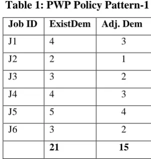
will be unallocated in a batch if this condition is satisfied. PWP Example–1

Table 1: PWP Policy Pattern-1

Job ID ExistDem Adj. Dem

J1 4 3

J2 2 1

J3 3 2

J4 4 3

J5 5 4

J6 3 2

21 15

In this table the figures shows that how PWP will modify the demand. Consider this Total No. of jobs 6, total batch demand 21 and if the current availability is 15. Then how PWP will adjust the existing demand.

Adjusted Demand for J1 is (4 * 15/21) = 60/21 = 2.8 = 3 Now total availability is 15-3=12

And total demand required 21- 4=17

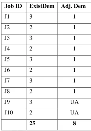
Note that J1 is now scheduled with 3 processors, its demand is modified. Like this calculates the demand for other jobs.Below isanotherexample showing the effect of PWP policy. In this example if second constraint fails the system willmake unallocation at the end. Consider we have 10 jobs in batch and we have total availability 8 and total batch demand is 25 then how PWP policy will behaves.

Table 2:PWP Policy Pattern-2

Job ID ExistDem Adj. Dem

J1 3 1

J2 2 1

J3 3 1

J4 2 1

J5 3 1

J6 2 1

J7 3 1

J8 2 1

J9 3 UA

J10 2 UA

25 8

Total Availability is 8 No. of jobs in the batch 10 Total Batch Demand is 25

So at most one processor is given to each job and two jobs at the end are unallocated.

Adjusted Demand for J1 is (3*8/25)=0.96 = 1, here note that if the metric result is less than 1 it will be awarded as 1 as described in this example.

Adjusted Demand for J2 is (2*7/22)=0.63=1

See above some jobs in the batch are scheduled but some at later are not scheduled. So in this situation the whole batch will not be scheduled until the given constraints are not satisfied. If batch is not scheduled the processors remain idle and the system waits for the allocated processors to free. Because size of the batch in terms of number of jobs is more than the current availability. Later the current research workwill focus on a new methodology based on selection of most optimal jobs from a batch for the current schedule if it is not possible to allocate the complete batch.

IV.

PRESENT

WORK

Present work performs optimal selection of jobs from a batch with the aim to maximize processor utilization. In the previous literature the research shows that demand of the processors will be modified in order to manage processor availability for the currently arrived batch. Also if given constraints are not satisfied the whole batch will be unallocated, so utilizing such idle processors via selection of most appropriate jobs from the batch which must maximize the overall computation. Batch partitioning is performed and remaining jobs are further handled along with next incoming batch and so on. In this way jobs are scheduled quickly and because of objective function of maximizing overall computation, the maximum throughput will be achieved.

several possibilities or feasible solutions exist but the need of optimality arises [8]. Later the research exhibits the use of knapsack programming approach to parallel scheduler for the selection of best optimal jobs set for the current availability.

Below are the general constraints of knap sack which will be redefined according to our parallel scheduler. 0-1 knapsack problem is followed in the scheduling, either the job is selected or not. In general given a set of n items each of which as a predefined weight and values. In addition a carry bag having a predefined capacity. So idea is to select most appropriate items from the set in order to maximize the overall value under limited weight capacity. This approach is manipulated to implement parallel schedulers where batch of jobs are arrived. Constraints of 0-1 knapsack problem.

Maximizing Value

(3)

Subject to

(4)

Where

Variable wj refers to the weight of jth item and variable pjdefines the value of the item j if included, this value should be maximized. Variable xj belongs to the values 0/1 if the item is included the xj denotes 1 other wise its value will be 0 meaning that item is not included. WC refers to the overall capacity under which the total weight should remains [8][9].

Redefining knapsack

knap sack can be redefined according to the parallel scheduler characteristics such as the variable WC can be represented as total availability of processors, that is the current available capacity of the system. Similarly the variable j can be used to represent job space. Like wise variable wjand pj can be used to represent demand and computation time of each job respectively. In this way, the parallel scheduler implemented for selection of optimal job set from a batch

V.

KNAPSACK

SCHEDULER

LAYOUT

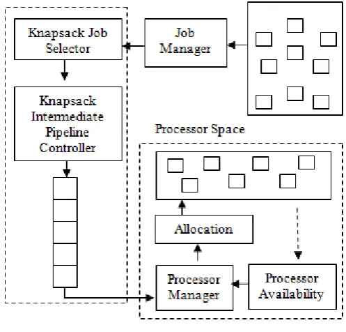
Knapsack approach to parallel scheduler plays an active role in computation speedup as well as throughput. Layout of the scheduling scheme exhibits a intermediate knapsack pipeline where the most optimal subset is placed before allocation. Basically a pre-fetch buffer which carries appropriate job set selected for the next allocation.

Fig. 1. Knapsack Scheduler Layout

Knapsack pipeline acts as a pre-fetch buffer for handling selected job set for the next schedule, the frequency of knapsack job selector is fast as compare to processor manager. Knapsack pipeline initially empty but as the pipe fills it always carrying a subset as early as possible for the next allocation. Processor space refers to the currently available processors where as job space refers to the batch arrivals.

VI.

PARAMETERIC

TERMS

DPM – Demand Promising Model, specifies that fixed demand allocation. In other words job’s demand must be full filled during allocation. Processing deeds should not be modified or moldable structure is not applicable. If current methodology follows the DPM model the thread level parallelism ultimately increased [1].

OEET – overall execution end time, deals with the total time taken at the end of the simulation. No. of batches are arrived and get their scheduling active using knapsack methodology. This metric will measure the system response that is how fast the simulation completes [1].

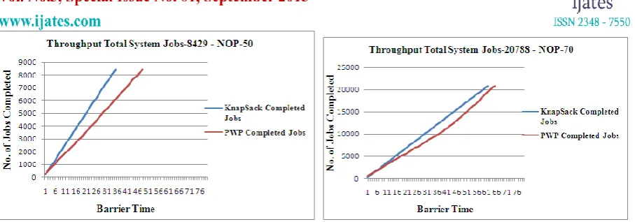
Throughput – This measure provides the no. of jobs completed in each time barrier. As the no. of jobs completed are more it will increase the system performance

VII.

SIMULATION

VIEW

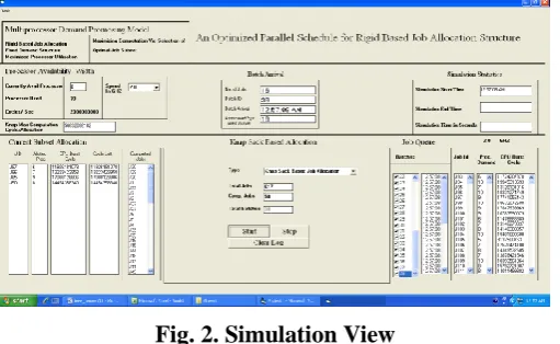
Fig. 2. Simulation View

Parallel scheduler plays an active role in job distribution. Scheduler operates according to a particular scheduling schemes employed and no. of processors available during that time. Several scheduling schemes exists, motivation is to allocate processors, best suited to current need/availability.

Simulator incorporates multithreaded environment. Batch arrivals are carried out by one thread where as one thread handles knapsack job selector and intermediate pipeline controller. Job allocation and completion will be handled by another thread. Finally simulation status measurement controls the system clock. Simulation results are recorded periodically at some barrier point. Later the PWP results are compared with KNP (Knapsack Parallel Scheduler).

VIII.

RESULTS

AND

DISCUSSIONS

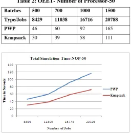
Results are carried out by running simulation after executing different samples. Each sample contains synthetic workload. Number of batches arrived and knapsack scheduler performs sub set selection and fills the intermediate pipeline. Below is the graph describing overall execution ending time using PWP and knapsack based scheduler. Simulation executed withvarying number of samples containing different number of batches each of which has different number of jobs. Analysis results exhibits how fast the knapsack scheduler is-

Table 3: OEET-Number of Processor-30

Batches 500 700 1000 1500

Type/Jobs 8429 11038 16716 20788

PWP 66 84 118 165

Fig. 3. Total Simulation End Time-NOP-30

The above graph exhibits that PWP policy structure has increased overall execution end time. Below is the another example showing similar effect of increasing number of processors. Existing literature about PWP also shows this effect. PWP adapts more moldable structure which leads to the response time delay. Although process level parallelism PLP will be increased in PWP as compare to knapsack. But PWP does not full fill the constraints of demand promising model. Further average processor utilization in each unit of allocation is described. As the batch arrived and gets scheduled total number of processor allocated, free as well as number of completed jobs at current timer barrier are stored in the system log which will be analyzed later on. As the model performs demand satisfaction, this will increase thread level parallelism as compare to PWP which using moldable approach of demand adjustments to manage best processor availability.

Table 2: OEET- Number of Processor-50

Batches 500 700 1000 1500

Type/Jobs 8429 11038 16716 20788

PWP 46 60 92 165

Knapsack 30 39 58 111

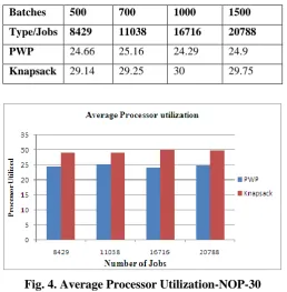
Table 4: Average Processor Utilization- NOP-30

Batches 500 700 1000 1500

Type/Jobs 8429 11038 16716 20788

PWP 24.66 25.16 24.29 24.9

Knapsack 29.14 29.25 30 29.75

Fig. 4. Average Processor Utilization-NOP-30

Average processor utilization computed by taking simulation results from the very beginning to till the end of simulation. No of processor allocated in each cycle. As the properties of knapsack describe optimal selection of sub set in each cycle, so knapsack provides better results than PWP.

Throughput is another factor of measuring system performance. PWP throughput is measured from the simulation and then compared with the throughput of knapsack scheduler. Below are the graphs that will exhibits throughput achieved by both the systems.

IX.

CONCLUSION

AND

FUTURE

WORK

The work done in this research incorporates rigid behavior of parallel workload that is demand of jobs will not be modified at any cost. As the literature describes sometimes it is not possible to allocate the complete batch corresponds to the current availability of processors. So its is required to focus on sub set selection from the batch that is more optimal selection of job set from the current batch, this will maximizes the performance of the system. As the illustrations describes overall throughput of the knapsack scheduler is more that PWP scheduler. Similarly average processor utilization is more in case of knapsack scheduler, not the full utilization some of the times this is because during subset selection it might be possible that there is no job available in the batch which has demand corresponds to current availability. Small processing limits may sit idle this is because no job having demand corresponding to available limit is available. Future work of this scheme must contain improvement to the current work. As the no. of processors are increases in the scheduler the process of knapsack subset selection is going to be slow. So the knapsack controller activities may be partitioned into multiple pipelines.

Table 4: Comparative Analysis

FACTOR/

POLICY

SDF EEMA

M-LIDA

PWP KNP

PLP Ex-Low Low High

Ex-High

High

TLP Ex-High High

Ex-High Ex-Low

Ex-High

Throughput Low High

Ex-High

Ex-low Ex-High

DPM Ex-High High High Ex-low

Ex-High

OEET High Low Low Ex-

High Ex-low APU

Average Processor Utilization

High High High High

Ex-High

MS -Moldable Structure Low Low High

Ex-High

As per the comparison described above, KNP approach is the best suited policy for the rigid based job allocation structure, where no need of demand changing exist at any cost. Moldable approaches follows demand modification so leads to the maximization of process level parallelism but over all throughput may be low due to the job execution at less no. of processors. Bon the other hand knapsack based scheduler performs best processor utilization as well as it follows demand promising model of computation. Overall execution end time also decreased as compare to other policy set.

REFERENCES

[1] S. Bagga, D. Garg “Moldable Load Scheduling Using Demand Adjustable Policies” ICACCI-2014 Galgotia Noida, IEEE Xplore, pp. 143-150.

[2] G. Sabin, M. Lang “Moldable Parallel Job Scheduling Using Job Efficiency: An Iterative Approach”12 international workshop JSSPP 2006, Springer Berlin, Saint Malo, France, pp. 94-114.

[3] K. Huang“Moldable Job Scheduling for HPC as a Service with Application Speedup Model and Execution Time Information” Journal of Convergence, Vol. 4, December 201, pp. 14-22.

[4] J. Moscicki “Processing Moldable Tasks on the Grid: Late job binding with light weight user-level overlays” in Elsevier Science, Publisher B. V. Amsterdam, The Netherlands, 2011, pp. 725-736.

[5] M. Etinski “Parallel Job Scheduling for Power constrained HPC systems”, Elsevier Science, B. V. Amsterdam, The Netherlands, 2012, pp. 615-630.

[6] A. Stephen, P. Daniel “Dynamic Scheduling of Parallel Jobs with QOS demand in Multi-Cluster and Grid” University of Warwick, 5th IEEE/ACM international Workshop on Grid Computing 2004, pp. 402-409 [7] V. Nguyen, R. Kirner “Demand Based Scheduling Priorities for Performance Optimization of Stream

Programs on Parallel Platforms” 13 International Conference, ICA3PP 2013, Springer Berlin Proceeding Part-1 18-20.

[8] S. Kolliosopoulos, G. Steiner “Partially Ordered Knapsack and Application to Scheduling”, Elsevier 2007, Vol. 155, issue 8. pp. 889-897.