127 | P a g e
DEVELOPMENT AND APPLICATION OF
MULTIOBJECTIVE FUZZY WASTE LOAD
ALLOCATION MODEL
Dr. K. Pavan Kumar
Department of Civil Engineering, SMBS, VIT Vellore, (India)
ABSTRACT
Water quality management though a very important part of overall water resources management programs is
also unfortunately given the last priority among all the other objectives like water supply for irrigation, drinking
purpose, hydropower, flood mitigation etc. In the present paper a multiobjective waste load allocation
(MOWLA) model has been developed. Though there are many MOWLA models with cost minimization and DO
maximization, there are very few models which have adequately addressed the issues of equity in waste load
allocation models. The present paper includes equity as one of the objective and shows that by introducing
equity in the objective function the solution obtained is more fair when compared to the overall cost
minimization solution. However the decision maker has different satisfaction levels to different solutions. To
address this uncertainty or ambiguity in a decision maker’s (DM) satisfaction level, fuzzy membership functions
are introduced for each objective function. thus by introducing fuzziness in the objective functions, a modeler
can give a wide range solutions from which the DM can select the most satisfying solution for himself.
Keywords:
Water Quality Management, Waste Load Allocation, Multi Objective Programming,
Fuzzy Logic
I.
INTRODUCTION
128 | P a g e
129 | P a g e
Mujumdar (2005)[14] developed a risk minimization model to minimize the risk of low water quality along a river in the face of conflict among various stake holders. Probabilistic Global Search Laussane (PGSL), a global search algorithm developed recently, was used for solving the resulting non-linear optimization problem. From the literature reviewed so far it appears that there is a scope in WLA problems where the issues of both fuzziness and randomness in model formulation can be addressed and incorporated. Saadatpour and Afshar (2007) [15] developed a simulation-optimization model for waste load allocation problem. For simulating the effects of pollutant load at a downstream point they used QUAL 2E and results obtained thus by were coupled with GA (genetic algorithm) optimization model. Singh et. al. (2007)[16] applied interactive fuzzy multiobjective linear programming model for finding BOD removal rates for each discharger located along river Yamuna.
II. DEFINING OBJECTIVES AND CONSTRAINTS
This section provides a brief overview of the methodology involved in the model development. The waste load allocation model was solved as a bi-objective optimization model. The objectives considered were, minimization of overall treatment level and maximization of equity. The objective functions Z1(x) and Z2(x) are
defined below.
Objective 1:- Minimization of overall treatment level, which is given by:
Where xi is the treatment level for an individual discharger i and n is the total number of dischargers.
Objective 2:- Maximization of equity for each discharger. Before formulating the objective function for equity, a brief overview on the concept of equity would be appropriate in understanding the equity objective function. Johnson (1967)[17], defined equity as a criterion where equals would be treated equally and non-equals would be treated differently i.e. dischargers who are discharging nearly same amount of effluent should be given same treatment levels, and all others should be given different treatment levels. Equity can also be defined based on the criterion that:
“The treatment level for each discharger should be equivalent to the product of the total effluent share of an individual discharger and the overall treatment removal for the system.”
Following above definition the objective function for equity can be given as:
where mi is the effluent BOD (after treatment) for an individual discharger, M is the total effluent BOD load
(after treatment) entering into the river and is given by
1 n
i i
m
and X is the overall treatment level of the systemgiven by
1 n
i i
x
130 | P a g e
2.1 Constraints for satisfying the maximum allowable DO deficit at a checkpoint (as a function of treatment levels):
Aimis a constant at a checkpoint m, for reach i, and it is a function of initial BOD of the river
Bimis a constant for a checkpoint m, within a reach i, and it is a function of effluent BOD entering the river reach.
The above constants are obtained by using Streeter-Phelps (1925) [18] equations and they show the effect on downstream DO deficit due to release of a unit point load at any upstream point.
2.2 Constraints on maximum and minimum treatment levels:
where xmin and xmax are the minimum and maximum treatment levels within which the treatment levels for each discharger would be fixed. For the present study, xmin has been taken as 0.3 and xmax as 0.9, except for D6 (sixth discharger) for whom xmax has been taken as 0.95, by virtue of his releasing nearly half of the total effluent load.
III. STUDY AREA DESCRIPTION
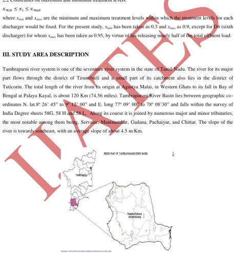
Tambraparni river system is one of the seventeen river system in the state of Tamil Nadu. The river for its major part flows through the district of Tirunelveli and a small part of its catchment also lies in the district of Tuticorin. The total length of the river from its origin at Agastya Malai, in Western Ghats to its fall in Bay of Bengal at Palaya Kayal, is about 120 Km (74.56 miles). Tambraparani River Basin lies between geographic co-ordinates N. lat.8º 26’ 45” to 9º 12’ 00” and E. long 77º 09’ 00” to 78º 08’30” and falls within the survey of India Degree sheets 58G, 58 H and 58 L. Along its course it is joined by numerous major and minor tributaries, the most notable among them being, Servalar, Manimutthar, Gadana, Pachaiyar, and Chittar. The slope of the river is towards southeast, with an average slope of about 4.5 m/Km.
Figure 1 Layout Map of Tambraparni River Baisn
131 | P a g e
3.1 Environmental Status of Tambraparni River
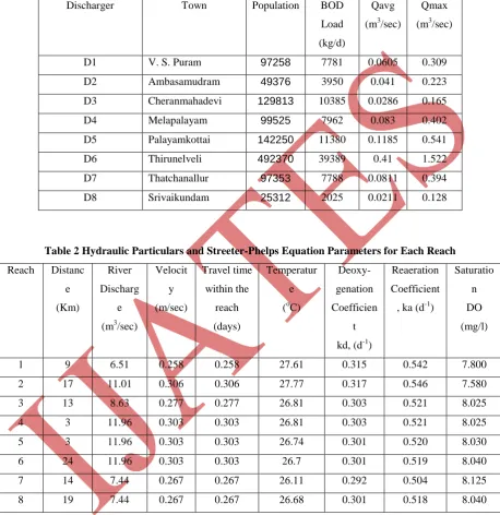
The major sources of pollution in the river are industrial effluent, domestic sewage and agricultural runoff. However there are very few major industries in the river basin, the major ones being Madhura Coats at V.S.Puram, and Sun Paper Mills at Cheranmahadevi. The major share of pollution in the river is due to uncontrolled disposal of domestic sewage and non point source pollution from agricultural runoff. There are no existing treatment plants for any of the major or minor towns in the river basin. This makes the effect of domestic sewage on the river water quality even more pronounced. Most of the small towns and villages in the basin area have no drainage (sewerage) facilities. The only towns which have partial sewerage system are Tirunelveli, V.S.Puram, Ambasamudram, Cheranmahadevi, Palayamkottai, Melapalayam and Srivaikundam. However The Government of India has sanctioned about Rs. 700 millions to implement underground sewerage system in Tirunelveli Corporation area (Microlevel Status Report for Tambraparni River Basin, 2003[19]). The DO in the river varies from a lowest value of 1.7 mg/l during the month of March to a highest value of 6.8 mg/l during the monsoon seasons of August and September whereas the BOD varies from 0.13 mg/l to 10.2 mg/l. Figure 2 below shows various towns located along the river which are discharging their domestic sewage directly into the river.
Figure 2 Index Map for Tambraparni River
VI. MODEL APPLICATION TO THE CASE STUDY
1. In the development of models for water quality certain assumptions need to be made and they are:
2. The population details obtained from Tamil Nadu Census Board were as upto the year 2001. However the present study is carried out for a projected population as on year 2010 with an assumption of a linear growth rate of 2% for all towns.
3. The daily per capita water consumption is taken as 90 lpcd and the waste water volume that reaches the river is assumed to be 80% of 90 lpcd.
4. The BOD load per person is taken to be about 0.08 kg/day.
132 | P a g e
Table 1 below gives the summary of the population detail, BOD load (kg/d), and effluent discharge for each town and Table 2 gives the particulars for the river.
Table 1 Population, BOD Load and Effluent Flow Rate Details for Each Town
Discharger Town Population BOD Load (kg/d)
Qavg (m3/sec)
Qmax (m3/sec)
D1 V. S. Puram 97258 7781 0.0605 0.309 D2 Ambasamudram 49376 3950 0.041 0.223 D3 Cheranmahadevi 129813 10385 0.0286 0.165 D4 Melapalayam 99525 7962 0.083 0.402 D5 Palayamkottai 142250 11380 0.1185 0.541 D6 Thirunelveli 492370 39389 0.41 1.522 D7 Thatchanallur 97353 7788 0.0811 0.394 D8 Srivaikundam 25312 2025 0.0211 0.128
Table 2 Hydraulic Particulars and Streeter-Phelps Equation Parameters for Each Reach
Reach Distanc e (Km)
River Discharg
e (m3/sec)
Velocit y (m/sec) Travel time within the reach (days) Temperatur e (oC)
Deoxy- genation Coefficien
t kd, (d-1)
Reaeration Coefficient
, ka (d-1)
Saturatio n DO (mg/l)
1 9 6.51 0.258 0.258 27.61 0.315 0.542 7.800 2 17 11.01 0.306 0.306 27.77 0.317 0.546 7.580 3 13 8.63 0.277 0.277 26.81 0.303 0.521 8.025 4 3 11.96 0.303 0.303 26.81 0.303 0.521 8.025 5 3 11.96 0.303 0.303 26.74 0.301 0.520 8.030 6 24 11.96 0.303 0.303 26.7 0.301 0.519 8.040 7 14 7.44 0.267 0.267 26.11 0.292 0.504 8.125 8 19 7.44 0.267 0.267 26.68 0.301 0.518 8.040
V. MODEL DEVELOPMENT
133 | P a g e
(1970)[21] min-max function can be used to convert the fuzzy multiobjective program into a fuzzy LP model, which can be then solved using any of the traditional LP optimization techniques. Before proceeding to solve the model we have to first develop membership functions for each objective functions. To develop membership function for an objective function, the model is first solved as a single objective optimization model for the given set of constraints, by both maximizing and minimizing the objective function for which the membership function is to be developed. During this operation other objective functions are kept as constraints. Thus for each objective function, we can find max and min values by following the above procedure. Once the max and min values for each objective functions are obtained, the membership functions for each objective function can be given as below (assuming that the variation of objective function from max to min is linear):
If the objective function is minimization, then the membership function is given as:
However if the objective function is maximizing, the membership function is given by:
For the present problem, the membership functions for the objective function of minimizing treatment removals and maximizing the equity were obtained as:
The membership function for the objective function of maximizing the equity was obtained as:
134 | P a g e
The fuzzy decision making problem now can be written as:
1 2 1 min max
[
{ ( ),
( )}]
:
;
1,...,
kim im i i
i
i i i
Max Min
x
x
subject to
A
B x
d
k
n
x
x
x
Where the terms have the same meaning as described in section (number). The above model can be converted into a fuzzy linear programming model as shown below:
1 2 1 min max
min
:
( )
( )
;
1,...,
0
1
0
1
i i kim im i i
i
i i i
i
subject to
x
x
A
B x
d
k
n
x
x
x
where γ is the minimum deviation that can be allowed from the reference membership function (RMF)
i. The above problem thus becomes a simple LP model which can be solved using any of the available programming software.VI. STEPWISE PROCEDURE FOR SOLVING THE FMOLP MODEL
Step 1:- Define the objective functions and constraints.
135 | P a g e
Step 3:- Once the maximum and minimum for each objective function are obtained, we can elicit a membership function for each objective function. The membership function should be non-increasing (non-decreasing) for minimization (maximization) objective function.
Step 4:- Using min-max fuzzy decision making function, the problem can be converted into a linear programming model where the objective is to minimize the maximum difference, γ between the RMF and membership function of the respective objective function.
Step5:- The model can be solved for different RMF values for each objective, whereby we will obtain a set of Pareto-optimal solution, from which the decision maker can choose an appropriate solution.
VII. RESULTS AND DISCUSSION
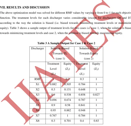
The above optimization model was solved for different RMF values by varying it from 0 to 1 for each objective function. The treatment levels for each discharger varies considerably (except for dischargers D6 and D7) according to the way the solution is biased (i.e. biased towards minimizing treatment levels or maximizing equity). Table 3 shows a sample output of treatment levels for two cases i.e. case 1, when the solution is biased towards minimizing treatment levels and case 2, when the solution is biased towards maximizing equity.
Table 3 A Sample Output for Case 1 & Case 2
Discharger Solution Biased Towards TL
(case 1)
Solution Biased Towards Equity
(case 2) Treatment
Level (Z1)
Equity (Z2)
Treatment Level
(Z1)
Equity (Z2)
RMF 1 0.3 0.3 1 X1 0.882 0.505 0.784 1 X2 0.3 0.131 0.648 1 X3 0.9 0.538 0.858 0.827 X4 0.696 0.674 0.787 1 X5 0.9 0.58 0.841 1 X6 0.95 0.882 0.948 1 X7 0.767 1 0.784 1 X8 0.3 0.701 0.4 0.83
136 | P a g e
Figure 4 Treatment Levels for Each Discharger for Case 1 and Case 2However by varying the RMF values for each objective function, a set of Pareto-optimal solution can be obtained for treatment levels and equity, from which the decision maker can select a solution which satisfies him on both treatment levels and equity.
VIII. CONCLUSION
A FMOLP model was developed for determining the treatment removal levels for each discharger in order to maintain the water quality of river Tambraparni. The objective functions for model were minimization of treatment levels for each discharger and maximization of equity among the dischargers.
When equity is not considered in the model, the treatment levels among the dischargers are distributed unevenly i.e. the treatment levels for each dischargers are not proportional to the percentage waste they are contributing into the river. Hence to overcome this type of inequity among the discharger, the objective function of maximizing equity was introduced. However maximization of equity led to increase in overall treatment level for the system, thereby increasing the overall treatment cost. To balance these two objectives, a set of compromise solutions were obtained, from which the decision maker can select a solution suitable for him.
137 | P a g e
It should be however noted that just these two objective functions are not enough for bringing water quality to the desirable level. Another objective of maximizing the BOD load for a discharger can be included in the optimization model, through which the DO deficit can be reduced still further from permissible limit.
REFERENCES
[1] Loucks, D. P., S. C. Revelle, W. R. Lynn. 1967. “Linear Programming Models for Water Pollution Control”. Management. Sci. 14, 13166-B181.
[2] Revelle S. C., D. P. Loucks., W. R. Lynn. 1968. “A Management Model for Water Quality Control”.
Water Resources Res. 39(7).
[3] Graves,G . W., G. B. Hatfielda ND A. Whinston. 1969. “Water Pollution Control Using By-pan piping”.
Water Resources Res. 5 ( 2 ) ,February.
[4] Liebman J. C., W. R. Lynn. 1966. “The Optimal Allocation of Stream Dissolved Oxygen”. Water Resources Res. 2(3), July.
[5] Cardwell, H., Ellis. H, (1993). “Stochastic dynamic programming for water quality management.” Water Resources Research, 29(4), 803-813.
[6] Ecker,J. G. 1975. “A Geometric Programming Model for Optimal Allocation of Stream Dissolved Oxygen”. Mgmt. Sci. 21, 658-668.
[7] Jowitt, P.W., and Lumbers, J. P. (1982). “Water quality objectives, discharge standards and fuzzy logic.”
Optimal Allocation of Water Resources (Proceedings of the Exeter Symposium, July 1982). IAHS Publ. no. 135, pp 241-250.
[8] Tung, Y. K., and Hathhorn, W. E., (1989). “Multiple-objective waste load allocation.” Water Resources Management, Vol. 3, pp 129-140.
[9] Benoit Julien., (1994). “Water quality modeling with imprecise information.” European Journal of Operational Research Vol. 76, pp 15-27.
[10] [Ni-Bin Chang and H. W. Chen., (1996). “The Application of Genetic Algorithm and Nonlinear Fuzzy Programming for Water Pollution Control in a River Basin.” IEEE, Vol. 9/96, pp 224-229.
[11] Chih-Sheng Lee, Ching-Gung Wen. (1996). “River assimilative capacity analysis via fuzzy linear programming.” Fuzzy Sets and Systems Vol. 79, pp 191-201.
[12] Sasikumar K. and Mujumdar P. P., (1998). “Fuzzy optimization model for water quality management of a river system”, J. Water Resour. Plann. Manage. Div., Am. Soc. Civ. Eng., 124, pp 79-88.
[13] Mujumdar P. P. and Sasikumar K., (2002). “A fuzzy risk approach for seasonal water quality management of a river system”, Water Resour. Res., 38(1), pp 5-1 – 5-9.
[14] Ghosh, S., Mujumdar, P.P., (2005). “Risk Minimization Model for River water Quality management”.
International Confernece on Hydrological Perspectives for Sustainable Development, HYPESD 05, IIT Roorkee, pp- 932-940.
[15] Saadatpour, M and Afshar, A., (2007). “Waste Load Allocation Modeling With Fuzzy Goals; Simulation-Optimization Approach.” Water Resources Management, 21(7), 1207-1224.
138 | P a g e
Research, 3, 291-305.[18] Streeter, H. W., and Phelps, E. B. (1925). “A study of the pollution and natural purification of the Ohio river. III: Factors concerning the phenomena of oxidation and reaeration.” Public Health Bulletin No. 146, U.S. Public Health Service, Washington, D.C.
[19] Fair, Gordon Maskew, Geyer, John Charles; Okun, Daniel Alexander “Water and Wastewater Engineering; Volume 1: Water Supply and Wastewater Removal”, John wiley and Sons, 1966.
[20] R. E. Bellman and L. A. Zadeh (1970). Decision making in a fuzzy environment. Management Science,