Modification of Symmetry of Poloidal Eigenmode of Geodesic
Acoustic Modes
Makoto SASAKI, Kimitaka ITOH
1), Akira EJIRI
2)and Yuichi TAKASE
2)Graduate School of Science, The University of Tokyo, Tokyo 113-0033, Japan
1)National Institute for Fusion Science, Toki 509-5292, Japan
2)Graduate School of Frontier Sciences, The University of Tokyo, Kashiwa 277-8561, Japan
(Received 28 April 2007/Accepted 8 January 2008)
The poloidal eigenmode of the geodesic acoustic mode (GAM) is analyzed in the case of high aspect ratio circular plasmas, and an analytic representation for poloidal eigenfunction is derived. Them=±1 andm=±2 (m
is the poloidal number) components of eigenfunction show up-down antisymmetry and up-down symmetry, re-spectively, in a torus. The mixing of the up-down symmetric and antisymmetric components becomes significant, when the ion gyroradius is large or when electron temperature is higher than ion temperature.
c
2008 The Japan Society of Plasma Science and Nuclear Fusion Research
Keywords: zonal flow, geodesic acoustic mode, eigenmode, eigenfrequency, eigenfunction, density oscillation, collisionless damping, gyrokinetic equation
DOI: 10.1585/pfr.3.009
1. Introduction
Recently, zonal flows (ZFs) have attracted much at-tention in plasma research. In particular, ZFs are thought to suppress anomalous transport in toroidal plasmas, and they also play an important role in turbulent transport [1–4]. ZFs are symmetric flows on a magnetic surface (the toroidal mode numbern =0 and the poloidal mode num-berm is very close to zero), which change their sign in the radial direction and their frequencyω is nearly equal to zero. In toroidal plasmas, an oscillation symmetric mode (n = 0,m ≈ 0) exists in addition to a static ZF. This mode arises from a nonzero divergence of theE×B
drift velocity, because a magnetic field line does not corre-spond to a geodesic line. This oscillating mode is called a geodesic acoustic mode (GAM) [2, 5, 6] , which was found by Winsoret al., using a fluid model [6]. Subsequently, a dispersion relation of the GAM was derived [7, 8]. Hinton
et al. analyzed GAM using the gyrokinetic equation, and discussed the partition ratio of the initial impulse between GAM and ZFs [9]. GAM oscillations are associated with a small but finite m = 1 component, therefore they are damped by ion Landau damping. In addition to these stud-ies, a strong collisionless damping by a finite orbit width (finite gyroradius) was studied [10, 11], and the GAM the-ory was extended to helical systems [10, 12, 13]. The non-linear excitation mechanism of GAM was also studied. In Refs. [14, 15], the excitation of GAM by turbulence was confirmed using direct numerical simulation (DNS). Ac-cording to a simulation, the excitation of GAM was at-tributed to the combination of the geometrical curvature and turbulent shear [16], based on which the condition for excitation of GAM due to microscopic turbulence was
de-author’s e-mail: [email protected]
rived [17]. These studies showed that GAM was excited by turbulence in configurations with higher safety factors. In parallel with these theoretical findings, the fluctuations of density and potential of GAM were recently observed in experiments, using Heavy Ion Beam Probe and electro-static probe, and a Doppler reflectometer [18–21]. These experimental observations require an accurate theoretical prediction of the temporal-spatial structure of the GAM eigenfunction.
The spatial structure of the GAM eigenfunction was studied based on these factors. The gyrokinetic equation and the quasi neutral condition served as the basic equa-tions. We considered poloidal modes up to them = ±2 components. The product of the radial wave numberkof the zonal flow and the ion gyroradiusρwas assumed to be much smaller than unity. Them=±1 andm=±2 compo-nents have different parity in the up-down symmetry, thus influencing the symmetry property of the eigenmode. The up-down symmetric components become large when either the ion gyroradius is large or when electron temperature is higher than ion temperature.
The outline of this article is as follows. In Sec. 2, the model and basic equations are introduced, and the response function to the fluctuation in potential is derived. In Sec. 3, the eigenequation is derived, and from it the eigenvalue [11] (which represents GAM frequency and damping rate) and the eigenfunction are obtained. Further, the poloidal structure of GAM potential is derived. The results obtained were comparable to those of previous studies. A discussion and summary are provided in Sec. 4.
c
2. Model and Basic Equation
2.1
Model
The configuration under study is assumed to be a high aspect ratio tokamak with a circular cross-section. Devi-ations from the circular cross-section, such as elongation and triangularity are not considered in this study. The mag-netic field can be expressed as
B= B0
1+cosθ
eζ+ qeθ
, (1)
whereeζ andeθ are the toroidal and poloidal directions, respectively,represents the inverse aspect ratio andqis the safety factor.
We derive a dispersion relation under the collisionless condition. The gyrokinetic equation and the quasi-neutral condition serve as the basic equations [22, 23]:
∂
∂t +vb· ∇+ik⊥·udr
δfk⊥
=−vb· ∇+ik⊥·udr×
F0J0(k⊥ρ)
eφk⊥
T
, (2)
dv3J0δf(i)
k⊥ −n0
1−Γ0(k2ρ2/2)eφk⊥ Ti = n0
Te
φk⊥− φk⊥
. (3)
Here, δfk(i)
⊥ andφk⊥ are the ion distribution function and
electrostatic potential, respectively, and subscriptk⊥ rep-resents the wave vector of zonal flow. The electron den-sity fluctuation is assumed to be a Boltzmann distribution for the non-zonal component and zero for the zonal com-ponent. TeandTiare the electron, and ion temperatures, respectively. ·represents the magnetic surface average,
F0is a Maxwell distribution,J0(x) is a zeroth-order Bessel function,Γ0(k2ρ2/2)=I0(k2ρ2/2) exp(−k2ρ2/2) (whereI
0 represents a zeroth-order modefied Bessel function),ρiis the ion gyroradius, andbis a unit vector representing the magnetic field direction. In Eq. (2),vdrrepresents the ra-dial component of toroidal drift due to inhomogeneity in the toroidal field, which can be expressed as
vdr=Ω1er· b
v2 +μ
B m
×∇B
B
. (4)
Hereafter, we omit the subscripts in the following cases:
kr=k(kr kθ), andδfk⊥ →δf, φk⊥ →φ.
2.2
Response of the distribution function to
fluctuation in potential
Assuming that the particle orbits are circular, the toroidal drift can be written as
kvdr=− vT qR0
kuˆsinθ=−s vT qR0
ˆ v2
+ ˆ v2
⊥ 2
sinθ. (5) Here, we introduce the dimensionless variables ˆv=v/vT, and ˆv⊥ =v⊥/vT. and, define the smallness parameters =
kvTq
Ω , which represents the finite orbit width effect.
In order to derive the response of distribution function to fluctuation in potential, we transform Eq. (2) into
∂ ∂t +
v
R0q ∂ ∂θ
eikδ(θ)δf
=− v
R0q
J0(svˆ⊥/q)∂ ∂θ
F0eikδ(θ)φˆ (6)
where ˆφ= eφ/Ti. In Eq. (6)ikδ(θ) represents the doppler
shift due to the toroidal drift motion, which can be written as
kδ(θ)=kR0q v0
vdr≈s
ˆ v+ ˆv
2 ⊥ 2ˆv
cosθ. (7)
Next, we perform Fourier transformation about timet
and poloidal angleθas δf(θ)=
∞
m=−∞
eimθ−iωtδfm(ω), (8a)
ˆ φ(θ)=
∞
m=−∞
eimθ−iωtφˆm(ω). (8b)
We then obtain the response relations between the distri-bution and potential for the poloidal mode numberm=0 from Eq. (2), and form0 from Eq. (6)
iωδˆ f0= 1
2J0(sˆv⊥/q)kuˆ(δf−1−δf1+φˆ−1−φ1ˆ ),(9a) δfm=
l,l
J0(sˆv⊥/q)F0 ˆ v(m−l) ω−vˆ(m−l)i
l−l
×Jl(kδ1)Jl(kδ1)φm−l−l, (9b)
where ˆω is the normalized frequency defined as ˆω = ωR0q/vT. These equations represent the response of the distribution function to the potential. The terms such as {ˆv(m±l)/(ω−vˆ(m±l))}il−lJ
l(kδ1)Jl(kδ1) represent
toroidal coupling with thel-th mode. Equation (9b) allows coupling with infinite terms, however the combination of higher harmonics results in a higher order ofkρ.
There-fore, the infinite summation can be approximated by a fi-nite summation. We only consider terms up tom=±1 in the determination of the real frequency.
In addition to this truncation, the GAM possesses the following symmetries
δfm(v)=(−1)mδf−m(−v), (10a)
φm=(−1)mφ−m, (10b)
which allow simplification in calculation. In particular, δf2, andδf1, δf0can be written explicitly as
iωδˆ f0=C00φ0+C01φ1+C02φ2, (11a) δf1=C10φ0+C11φ1+C12φ2, (11b) δf2=C20φ0+C21φ1+C22φ2. (11c) The coefficientsCi j are discussed in Appendix A.
Eq. (3), which is a quasi-neutrality condition, we obtain the following equations:
in0ωˆ
s2 2q2φ0ˆ =
C00d3vφ0ˆ +
C01d3vφ1ˆ +
C02d3vφ2,ˆ (12a)
n0 1 τeφ1=
C10d3vφ0ˆ +
C11d3vφ1ˆ +
C22d3vφ2,ˆ (12b)
n0 1 τeφ1=
C20d3vφ0ˆ +
C21d3vφ1ˆ +
C22d3vφ2.ˆ (12c)
3. Eigenvalue and Eigenfunction
3.1
Eigenequation
In this section, we derive the explicit form of the eigenequation. Equations (12a-c) can be expressed in ma-trix form as follows:
⎛ ⎜⎜⎜⎜⎜
⎜⎜⎜⎜⎝ DD0010 DD0111 DD0212
D20 D21 D22 ⎞ ⎟⎟⎟⎟⎟ ⎟⎟⎟⎟⎠ ⎛ ⎜⎜⎜⎜⎜ ⎜⎜⎜⎜⎝ ˆ φ0 ˆ φ1 ˆ φ2 ⎞ ⎟⎟⎟⎟⎟
⎟⎟⎟⎟⎠=0. (13)
The coefficients in Eq. (13) can be derived as
D00=iωˆ
s2
2q2n0+n0i
s2
2 1 2ω+ˆ ωˆ
3+ωˆ4Z( ˆω)+ωˆ(1+ωˆZ( ˆω))
+i√πs
2
8
6 ˆ ω2 +3+
3 4ωˆ
2+ωˆ4 16+
ˆ ω6 64
e−ωˆ2/4
,(14a)
D01=n0sωˆ2+
1 2ωˆ +ωˆ
3
Z( ˆω) +i√πs
2
4
3 2 ˆω +
3 4ωˆ +
3 16ωˆ
3+ωˆ5 32
e−ωˆ2/4
, (14b)
D02=i 1 2ns
2 3 4ωˆ +
7 8ωˆ
3+
1 2 +ωˆ
2+ωˆ4
Z( ˆω)
−i√π
1 2+ ˆ ω2 4 + ˆ ω4 16
e−ωˆ2/4
, (14c)
D10=i
n0s 2 ωˆ +
ˆ ω2+1
2
Z( ˆω) +i√πs
2
8
3 ˆ ω2 +
3 2 3 8ωˆ
2+ωˆ4 16
e−ωˆ2/4
, (14d)
D11=n0 1
τe +n0 1+ωˆZ( ˆω) +i√πs2
1 ˆ ω + ˆ ω 2 + ˆ ω3 8
e−ωˆ2/4
, (14e)
D12=i 1 2n0s −
ˆ ω
2−
1 2+ωˆ
2
Z( ˆω)+i√π
1 2+ ˆ ω2 4
e−ωˆ2/4
,
(14f)
D20=− 1 8n0s
2 3 2+
ˆ ω2
4 +i
√ π 1 ˆ ω+ ˆ ω 2 + ˆ ω3 8
e−ωˆ2/4
,
(14g)
D21=i 1 2n0s
−ωˆ
2 −
1 2 +ωˆ
2
Z( ˆω)
+i√π
1 2+ ˆ ω2 4
e−ωˆ2/4
, (14h)
D22=n0 1 τe +n0i
√
π
1+ωˆ 2
e−ωˆ2/4. (14i) In order to clarify thes-ordering, we introducedi j, andei j
as
D0j=n0s2
d0j+s2e0j
, (15a)
Dj0=n0s2
dj0+s2ej0
(j=0,2), (15b)
Dii=n0
dj0+s2ej0
(i=1,2), (15c)
Di j=n0s
di j+s2ei j
(others). (15d)
Next, we derive the dispersion relation, which is the determinant ofDi j. We include only the real parts of terms
up toO(s2) and the imaginary parts of terms up toO(s4). The dispersion relation can be written as
Δ=s2
Δr+i
Δi0+s2Δi1 =0, (16)
whereΔrdetermines the real frequency of GAM,Δi0 rep-resents the fundamental property of GAM in terms of an imaginary frequency, andΔi1 represents the finite ion gy-roradius effect in terms of an imaginary frequency of the
s2-order. These terms are written as Δr0=Re
d00 d01
d10 d11
, (17a)
Δi0=Im
d00 d01
d10 d11
, (17b)
Δi1=Im
e00 e01
d10 d11
+ d00 d01
e10 e11 +
−d12
d22
d00 d01
d20 d21 +d02
d22
d10 d11
d20 d21 . (17c)
3.2
Eigenvalue
Here, we derive the fundamental eigenvalue by solv-ing the fundamental dispersion relation
Δr0+i
Δi0+s2Δi1
=0. (18)
Since, we are considering the GAM frequency, we apply the ˆω 1 approximation, and expand the plasma disper-sion function asymptotically. The expanded coefficients
di j, andei j are discussed in the appendix. The real
fre-quency is determined by substituting Δr0 = 0, and the imaginary part is assumed to be much smaller than the real part, i.e., ˆω γ. The fundamental dispersion relation isˆ approximated up toO( ˆγ), where ˆγcan be obtained as Δr0( ˆω+γ)ˆ +iΔi0( ˆω+γ)ˆ +s2Δi1( ˆω+γ)ˆ
≈Δr0( ˆω)+i
∂Δr0( ˆω0)
∂ωˆ γ+ˆ Δ0( ˆω)+s 2Δ
i1( ˆω)
=0 (19)
↔γˆ≈ −Δi0+s 2Δ
i1
Thus, the lowest order estimate forωcan be derived as ω0 =ω(0)
G +iγ (0)
G, (21)
ω(0) G =
7 4+τe
vT
R0
1+223+16τe+4τ 2 e (7+4τe)2q2
1/2 ,(22)
γ(0) G =−
√
πqτe vT
2R0
1+223+16τe+4τ 2 e (7+4τe)2q2
−1
× ωGˆ 41 τe+ωGˆ 2
1 τe+
3 2ωGˆ
2
e−ωˆG2 +1
8s 2e−ωˆG2/4
1 64τeωGˆ 6+
15 128 +8τe1 + 1
4q2
ˆ ωG4+
3 4τe+
93 256
ˆ ωG2
.(23)
In the above equations, the terms containing exp−ωˆ2 G/4
represent the Landau damping effect as pointed out by Sugama and Watanabe [11, 12]. The coefficient of exp−ωˆ2
G/4
in Eq. (23) has been modified, and the leading term is expressed as 1/8×1/64τe.
3.3
Eigenfunction
3.3.1 potential eigenfuction
The poloidal eigenfunction can be derived from the eigen equation Eq. (13). Here, we transform Eq. (13) into
D11 D12
D21 D22
φ1/φ0 φ2/φ0
=−
D10
D20
. (24)
From this equation, we can obtain φ1
φ0 =
D12D20−D22D10
D11D22−D12D21
≈i1
2
sτe
ˆ
ω , (25a)
φ2 φ0=
D21D10−D11D20
D11D22−D12D21
≈−s2τe
ˆ ω2
1 4τe+
7 8
. (25b) Considering the parity of Fourier components (φ−m =
(−1)mφm), the poloidal eigenfunction can be expressed as
φ(θ) φ0 =
m
eimθφm
≈1− sτe ˆ
ωGsinθ−
s2τe ˆ ωG2
1 2τe+
7 4
cos 2θ. (26) The value of the GAM potential is nearly constant on the magnetic surface, and dependence onθis introduced by a small but finite ion-gyroradius effect.
The signs of k and u are important when analyzing the spatial structure of the eigenfunction. The general wave (composed of traveling and the standing waves), can be ex-pressed by the superimposing waves that are propagating towardr >0 andr <0. Forω >0, we need to consider both positive and negative values ofk. In this paper, posi-tiveωis chosen as a convention. Here, the waves ofk>0 andk < 0 represent traveling waves propagating toward
r > 0 andr < 0, respectively. When the amplitudes of these components are the same, resulting wave represents a standing wave.
propagating wave First, we discuss the case of the uni-directional radially propagating wave. Here we consider
k>0. In this case, the spatial structure of the eigenfunc-tion can be written as
φ(r, θ)
φ0 ≈
1− sτe ˆ
ωGsinθ−
s2τe
ˆ ωG2
1 2τe+
7 4
cos 2θ
×cos(kr−ωGt). (27) As seen in Eq. (27), the structure determined by Eq. (26) propagates radially. The m = ±1 components has a sinθdependency, which shows an up-down antisymmetry against the midplane of the torus. Its amplitudekρqτe/ωGˆ depends on the sign of the phase of electric fieldk(when the direction of increase in E ×B drift velocity is posi-tive along thez-axis, the eigen function increases along the positivez-axis). The m = ±2 components have a cos 2θ
dependence, which has an up-down symmetry in the torus. Its amplitude is approximately∼ k2ρ2q2τ2e/ωˆ2
G, which is independent of the sign ofk. This component becomes larger when the ion gyroradius is large or when the elec-tron temperature is higher than the ion temperature; it is almost independent ofq because the leading term of ˆωG is proportional toq. In addition, them=±2 components always reduce the amplitude of them = 0 component at θ=0, πand they intensify atθ=±π/2. The amplitude of
m=±1 is intensified positively in the bottom of the torus (θ = 3π/2) by them =±2 components. The region sat-isfying the condition of|φ(θ)| < |φ0|widens. As seen in Eq. (26), them=±1 component can be deduced from the values ofφ(θ) atθ = π/4. Once them = ±1 component is determined, them =±2 component can be deduced by comparing theφ(θ) values atθ=0, π/2.
standing wave We now discuss the case of the standing wave. The lowest order term, i.e. them = 0 component, can be written as
φ(r, θ)
m=0
=φ0
expi(kr−ωGt) +expi(−kr−ωGt−iδ)
. (28)
In this case, the spatial structure of the eigenfunction can be written as
φ(r, θ)
φ0 ≈ 2−2
s2τe ˆ ωG2
1 2τe+
7 4
cos 2θ
×cosk
r− δ
2k
cosωG
t− δ
2ωG
+2sτe ˆ
ωGsinθsink
r− δ
2k
×sinωG
t− δ
2ωG . (29)
and space. Unlike the case of the propagating wave, the structure does not propagate radially, but oscillates tempo-rally. As Eq. (29) shows, the time and radial dependences ofm=±1 andm=±2 components differ from each other.
Therefore, the poloidal angle that satisfiesφ(θ) =φ0 at a certain radius changes with time. Furthermore, at a cer-tain time (t = δ/2ωG+nπ,n = 0,1,2. . .), them = ±1 components disappear, whereas them=0,±2 components remain. In contrast, at timet =δ/2ωG+(n+1/2)π, the m = 0,±2 components disappear, and only them = ±1 components remain. The structure has a radial periodicity of 2π/kwhen the time is fixed, and has a time periodicity of 2π/ωGwhen the radial position is fixed. Furthermore, in the case of the general wave, which can be expressed by superimposing the propagating and the standing waves, the effect of them =±2 components on them =±1 compo-nents vary radially.
3.3.2 density eigenfuction
Because the density eigenfunction is more easily ob-served, we explain the density fluctuation. The electron density fluctuation is obtained from Eq. (3), and is ex-pressed as
˜
n(θ) n0
=φ0ˆ
−sτe
ˆ
ωGsinθ−
s2τe ˆ ωG2
1 2τe+
7 4
cos 2θ
.
(30) Radially propagating and standing waves are reconstructed by choosing an appropriate sign fork.
propagating wave First, we discuss the case of the uni-directional radially propagating wave. Here we selectkas
k>0. In this case, the density structure of the eigenfunc-tion can be written as
˜
n(r, θ) n0
=φ0ˆ
−sτe
ˆ
ωGsinθ−
s2τe ˆ ωG2
1 2τe+
7 4
cos 2θ
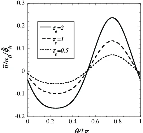
×cos(kr−ωGt). (31) It is found that theθdependent structure propagates radi-ally. The leading order of the density fluctuation is approx-imatelykρ, and shows sinθdependence, which is antisym-metric in the torus. Similar to the potential eigenfunction, them=±1 components depend on the sign ofk, whereas them=±2 components are independent of it. The behav-ior of density eigenfunction is shown in Fig. 1 for a fixed the time and radial position (kr−ωGt=2nπ,n=0,1,2. . .). Although the sign of the density eigenfunction changes in the vertical direction, the up-down antisymmetry is broken. To show the effect of breaking of antisymmetry, we analyze the ratio between the top and bottom, (i.e., ˜n(3π/2)
and ˜n(π/2), in Fig. 2), which is always unity when an-tisymmetry holds. It is found that ˜n(3π/2)/˜n(3π/2)
in-creases whenkρbecomes large, which indicates that the antisymmetry increases. When kρ ∼ 0.1, this antisym-metry is several tens of percent of the density fluctua-tion, which can be observed. In addifluctua-tion, we analyze the
Fig. 1 Eigenfunctions for severalτe(τe =0.5,1,2), withkρ=
0.1, andq=3.
Fig. 2 kρdependence of the asymmetry in density perturbation. Asymmetry is defined as ˜n(3π/2)/n˜(π/2), forq=3, and
τe=1.
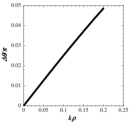
poloidal angles which the density fluctuation becomes zero at all times (these points are defined asθ0, andθ1). When
kρis small, the density fluctuation is nearly antisymmetric, resulting in zero points ofθ0=0, andθ1=π. However, if
kρbecomes larger, the antisymmetry breaks down, there-foreθ0, andθ1moves from 0, πto 0−Δθ, π+Δθ, respec-tively. The behavior ofΔθis shown in Fig. 3, in which it is possible to detect the density fluctuation at the midplane. The density perturbations for the (r, θ) plane are illustrated
Fig. 3 kρdependence of the points where the density fluctuation becomes zero, forq=3, andτe=1.
Fig. 4 Spatial structure of density fluctuation in propagating wave on the (r, θ) plane atωG(t−t0) = 2nπ, nis an
integer, andt0 = δ/2k. The solid line shows the
con-tour of ˜n/nφ0 >0, the dashed line shows the contour of
˜
n/nφ0 <0, and the dash-dot line shows the contours of
˜
n/nφ0=0.
standing wave Next, we discuss the case of the standing wave based on Eq. (28). Here, the spatial structure of the density eigenfunction can be written as
˜
n(r, θ)
n0 =
ˆ φ0
2sτe
ˆ
ωGsinθsink
r− δ
2k
×sinωG
t− δ
2ωG
−2s 2τe
ˆ ωG2
1 2τe+
7 4
×cos 2θcosk
r− δ
2k
cosωG
t− δ
2ωG . (32) As seen in this equation, the effect of them=±2 compo-nents onm =±1 components changes radially, similar to the potential eigenfunction. Unlike the case of the propa-gating wave, the region of ˜n/nφ0ˆ <0 changes both radially and temporally, which is shown in Fig. 5. The time origin
Fig. 5 Spatial structures of the density fluctuation in the stand-ing wave on the (r, θ) plane. (a) atωG(t−t0)=2nπ, (b) at
ωG(t−t0)=π/4+2nπ, (c) atωG(t−t0)=π/2+2nπ, and
(d) atωG(t−t0)=3π/4+2nπ. The solid line shows the
contour of ˜n/nφ0>0, the dashed line shows the contour
of ˜n/nφ0<0, and the dash-dot line shows the contours of
˜
n/nφ0=0.
is defined as the time when them =±1 components dis-appear,t =δ/2ωG+2nπ. This variation in the pattern of
the standing wave is compared to that of the propagating wave shown in Fig. 4. Theθ-dependent structure moves in ther-direction without changing its shape in the case of the propagating wave, whereas the pattern itself changes in the case of the standing wave.
Finally, we comment on the phase difference between ˜
nandφ, where we consider only the dominant terms for simplicity (i.e. them=0 component inφand them=±1 components in ˜n). It is observed that propagating waves have peaks at the same radial location (kr−ωGt = 2nπ),
whereas standing waves have peaks that shift radially by
kΔr=π/2.
4. Summary
In this study, the spatial structure of the GAM poloidal eigenfunction was analzsed. The analytical representations of the potential and density eigenfunctions were obtained. The eigenfunction of them=±1 components showed the up-down antisymmetry in the torus, and them=±2 com-ponents showed up-down symmetry in the torus. The mix-ing of the up-down symmetric and antisymmetric compo-nents becomes significant, when the ion gyroradius is large or when the electron temperature is higher than the ion temperature. The asymmetry defined by−n˜(3π/2)/˜n(π/2)
5. Acknowledgement
The authors thank Prof. H. Sugama and the reviewer of this paper for useful discussions. This work was partly supported by a Grant-in-Aid for Scientific Research (193604918), by a Grant-in-Aid for Specially-Promoted Research (16002005), by the Collaboration Program of NIFS (NIFS06KDAD005), and by the University of Tokyo 21st Century COE Program (200300G2).
Appendix A. Coe
ffi
cients (
C
i j)
The coefficients of the response of ion distribution to fluctuation in potential, from Eq. (11c), are obtained as
C00=− 1 2kuFˆ 0
1 2i(kδ)
ˆ v ˆ ω−ˆv +
ˆ v ˆ ω+ˆv
+ 1 16i(kδ)
3
2ˆv ˆ
ω−2ˆv+ 2ˆv ˆ
ω+2ˆv , (A.1)
C01=− 1 2kuFˆ 0
ˆ v ˆ ω−ˆv−
ˆ v ˆ
ω+vˆ +2 +1
4(kδ) 2
2ˆv ˆ
ω−2ˆv − 2ˆv ˆ
ω+2ˆv , (A.2)
C02=− 1 2kuFˆ 0
−1
2i(kδ)
2ˆv ˆ
ω−2ˆv + 2ˆv ˆ ω+2ˆv
− vˆ
ˆ ω−vˆ −
ˆ v ˆ ω+vˆ
+ 1 16i(kδ)
3
3ˆv ˆ
ω−3ˆv+ 3ˆv ˆ
ω+3ˆv , (A.3)
C10=F0
i1
2(kδ) ˆ v ˆ
ω−ˆv +i 1 16(kδ)
3 2ˆv ˆ ω−2ˆv
,
(A.4)
C11=F0
ˆ v ˆ ω−ˆv+
1 4(kδ)
2 2ˆv ˆ ω−2ˆv
, (A.5)
C12=F0
i1
2(kδ)
ˆ v ˆ ω−ˆv −
2ˆv ˆ ω−2ˆv
−i 1
16(kδ) 3 3ˆv
ˆ ω−3ˆv
, (A.6)
C20=F0
−1
8(kδ) 2 2ˆv
ˆ ω−2ˆv +(kδ)4
1 32
2ˆv ˆ
ω−2ˆv − 1 96
3ˆv ˆ
ω−3ˆv , (A.7)
C21=F0
i1
2(kδ)
2ˆv ˆ
ω−2ˆv − ˆ v ˆ ω−2ˆv
+i(kδ)3
1 16
3ˆv ˆ
ω−3ˆv− 1 6
2ˆv ˆ
ω−2ˆv , (A.8)
C22=F0
2ˆv ˆ ω−2ˆv +(kδ)2
−1
2 2ˆv ˆ
ω−2ˆv + 1 4
3ˆv ˆ
ω−3ˆv . (A.9)
Appendix B. Expansion of
d
i j, and
e
i jdi jandei jdefined in Eqs. (15a)-(15d) are coefficients
of the response of density fluctuation to fluctuation in po-tential. These coefficients haveZ( ˆω) terms. In the case of GAM, since ˆω 1 is satisfied, it is possible to expand
Z( ˆω). From this expansion,di jandei jcan be written as
d00≈iωˆ 1 2q2 −i
1 2 7 4 1 ˆ ω + 23 8 1 ˆ ω3
+i1
2i
√
π
ˆ
ω4+ωˆ2+1 2
e−ωˆ2, (B.1)
d01≈ −
1+ 1 ˆ ω2 +
1 ˆ ω4
+i√π1
2ωeˆ −ωˆ2
, (B.2)
d02≈i 1 2 7 4 1 ˆ ω + 161 8 1 ˆ ω3
−i√πe−ωˆ2/4
1 2 +
1 4ωˆ
2+ 1 16ωˆ
4 , (B.3)
d10≈i 1 2 − 1 ˆ ω + 1 ˆ ω3 +i√π
ˆ ω2+1
2 , (B.4)
d11≈ 1 τe− 1 2 1 ˆ ω2 +
3 4 1 ˆ ω4
+i√πωeˆ −ωˆ2, (B.5)
d12≈i 1 2 − 1 ˆ ω − 7 ˆ ω3 +i
√
π
1 4ωˆ
2+1 2
e−ωˆ2/4
,
(B.6)
d20≈ − 1 8
− 7
ˆ ω2−
46 ˆ ω4+i
√
πe−ωˆ2/4 1 ˆ ω+ ˆ ω 2+ ˆ ω3 8 , (B.7)
d21≈i 1 2 − 1 ˆ ω − 7 ˆ ω3 +i
√
πe−ωˆ2/4
1 4ωˆ
2+1 2 ,
(B.8)
d22≈ 1 τe−
2 ˆ ω2 −
12 ˆ ω4 +i
√
πωˆ 2e
−ωˆ2/4
, (B.9)
e00≈i 1 2
i√π1
8e −ωˆ2/4
6 ˆ ω2+3+
3 4ωˆ
2+ωˆ4 16+
ˆ ω6 64 ,
(B.10)
e01≈ 1 4i
√
πe−ωˆ2/4 3 2 1 ˆ ω+ 3 4ωˆ +
3 16ωˆ
3+ωˆ5 32
,
(B.11)
e10≈i 1 2 1 8 √
πe−ωˆ2/4
3 ˆ ω2 +
3 2 +
3 8ωˆ
2+ωˆ4 16 ,
(B.12)
e11≈i
√
πe−ωˆ2/4 1 ˆ ω+ ˆ ω 2 + ˆ ω3 8 . (B.13)
[1] P.H. Diamond, S.-I. Itoh, K. Itoh and T.S. Hahm, Plasma Phys. Control. Fusion47, R35 (2005).
[2] K. Itoh, S.-I. Itoh and A. Fukuyama,Transport and Struc-tual Formation in Plasma(IOP, 1999, Bristol).
[3] A. Yosizawa, S.-I. Itoh and K. Itoh,Plasma and Fluids Tur-bulence(IOP, 2002, Bristol).
[6] N. Winsor, J.L. Johnson and J.J. Dawson, Phys. Fluids.11, 2248 (1968).
[7] V.B. Lebedev, P.N. Yushmanov, P.H. Diamond, S.V. Novakovskii and A.I. Smolyakov, Phys. Plasmas3, 3023 (1996).
[8] S.V. Novakovskii, C.S. Liu, R.Z. Sagdeev and M.N. Rosenbluth, Phys. Plasmas4, 4272 (1997).
[9] F.L. Hinton and M.N. Rosenbluth, Plasma Phys. Control. Fusion41, A653 (1999).
[10] H. Sugama and T.-H. Watanabe, Phys. Plasmas13, 012501 (2006).
[11] H. Sugama and T.-H. Watanabe, J. Plasma Phys.72, 825 (2006).
[12] T. Watari, Y. Hamada, A. Fujisawa, K. Toi and K. Itoh, Phys. Plasmas12, 062304 (2005).
[13] S. Satake, K. Okamoto, N. Nakajima, H. Sugama, M. Yokoyama and C.D. Beidler, Nucl. Fusion45, 1362 (2005). [14] T.S. Halm, Plasma Phys. Control. Fusion42, A205 (2000). [15] K. Hallatschek, Phys. Rev. Lett.84, 5145 (2000).
[16] K. Hallatschek, Phys. Rev. Lett.86, 1223 (2001).
[17] K. Itoh, K. Hallatshek and S.-I. Itoh, Plasma Phys. Control. Fusion47, 451 (2005).
[18] A. Fujisawa, K. Itoh, H. Iguchi, K. Matsuoka, S. Okamura, A. Shimizu, T. Minami, Y. Yoshimura, K. Nagaoka, C. Takahashi, M. Kojima, H. Nakano, S. Ohsima, S. Nishimura, M. Isobe, C. Suzuki, T. Akiyama, K. Ida, K. Toi, S.-I. Itoh and P.H. Diamond, Phys. Rev. Lett. 93, 165002 (2004).
[19] Y. Nagashima, K. Hoshino, A. Ejiri, K. Shinohara, Y. Takase, K. Tsuzuki, K. Uehara, K. Kawashima, H. Ogawa, T. Ida, Y. Kusama and Y. Miura, Phys. Rev. Lett. 95, 095002 (2005).
[20] G.D. Conway, B.S. Scott, J. Shirner, M. Reich, A. Kendi and the ASDEX Upgrade Team, Plasma Phys. Control. Fu-sion47, 1165 (2005).
[21] T. Ido, Y. Miura, K. Kamia, Y. Hamada, H. Hoshino, A. Fujisawa, K. Itoh, S.-I. Itoh, A. Nishizawa, H. Ogawa, Y. Kusama and JFT-2M group, Plasma Phys. Control. Fusion
48, S41 (2006).
[22] E.A. Frieman and Liu. Chen, Phys. Fluids25, 502 (1982). [23] R.D. Hazeltine and J.D. Meiss, Plasma Confinement