Algebraic Analysis Approach for Multibody Problems II
Shun-ichi OIKAWA, Koichiro HIGASHI and Hideo FUNASAKA
a)Graduate School of Engineering, Hokkaido University, Sapporo 060-8628, Japan
(Received 6 January 2009/Accepted 8 June 2009)
The algebraic model (ALG) proposed by the authors has sufficiently high accuracy in calculating the motion of a test particle with all the field particles at rest. When all the field particles are moving, however, the ALG has relatively poor prediction ability on the motion of the test particle initially at rest. None the less, the ALG approximation gives a good results for the statistical quantities, such as variance of velocity changes or the scattering cross section, for a sufficiently large number of Monte Carlo trials. For a 108-body problem, which corresponds to full three-dimensional Coulomb interactions within the Debye sphere in a fusion plasma, the ALG approximation is 263 times as fast as the 6-stage 5-th order Runge-Kutta-Fehlberg method with an absolute error tolerance of 10−16.
c
2010 The Japan Society of Plasma Science and Nuclear Fusion Research
Keywords: multibody problem, algebraic approximation, binary interaction approximation, direct integration method
DOI: 10.1585/pfr.5.S1048
1. Introduction
Since it is difficult to rigorously deal with multibody Coulomb and gravitational collisions, the current classical theory considers them as a series of temporally-isolated bi-nary Coulomb and gravitational collisions within the De-bye sphere. The efficient and fast algorithms to calculate inter-particle forces include the tree method [1, 2], the fast multipole expansion method (FMM) and the particle-mesh Ewalt (PPPM) method [3]. Efforts have been made to use parallel computers, and/or to develop special purpose hardware to calculate interparticle forces, e.g. the GRAPE (GRAvity PipE) project [4]. Some of the authors have de-veloped an algebraic model for multibody problems, and have shown that the momentum transfer cross-section with our model is in good agreement with the exact one [5].
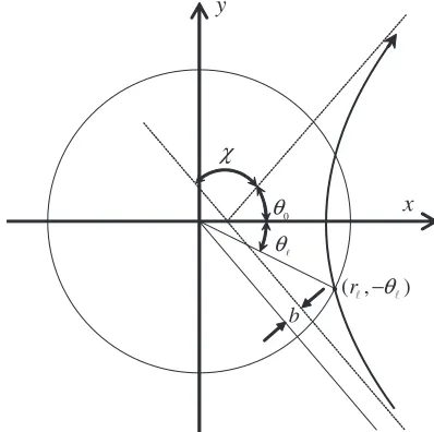
As shown in Fig. 1 the scattering angle,χ ≡π−2θ0,
is given byb=b0tanθ0, wherebis the impact parameter,
b0 ≡ e2/4πε0μg20 corresponds toχ = π/2 scattering, and g0 the initial relative speed atr = ∞andθ = −θ0. The
angular component of the equation motion gives the well-known invariant of
r2dθ
dt =const=bg0, (1)
and the radial component is given by d2r
dt2 = g2
0b0
r2
1+b0 r tan
2θ 0
, (2)
which can be analytically solved as r(θ)= bsinθ0
cosθ−cosθ0 .
The first term in the parentheses on the right hand side of author’s e-mail: [email protected]
a)currently with DENSO Corporation
Eq. (2) stands for the Coulomb forceFc∝r−2. This force
is much smaller for small angle scatterings, i.e.χ1, than the second termFawhich scales as∝r−3and results from
the conservation of angular momentum Eq. (1), since, at the closest pointrmin =r(θ=0) shown in Fig. 1, we have
b0tan2θ0
rmin
2χ 1. (3)
Thus the main force on the particle is not the Coulomb forceFc, but Fa due to the conservation of angular
mo-mentum.
Fig. 1 Unperturbed relative trajectoryr = r(θ) in an orbital plane for the repulsive force. The scattering center is at the origin. An impact parameter isb =b0tanθ0.
Inter-action region is inside the circle with a radiusr= Δ/2, whereΔstands for the average interparticle separation.
c
2010 The Japan Society of Plasma
2. Algebraic Approximation
Since ther-dependence on Fa ∝ r−3 is steeper than
that onFc ∝ r−2, the momentum change inμgis almost
due solely toFanearr=rmin. As a consequence, the exact
hyperbolic trajectory for the particle can be approximated as a broken line with an impulse force of
μΔg=2μg0cosθ0ex, (4)
near the closest point as shown in Fig. 2.
With this in mind, we have approximated a multibody problem to a series of binary deflections near their closest point as shown in Fig. 2, in which a test particle starts at the lower-right point, and its final point is at the upper-right point due to the interaction with a field particle at rest.
2.1
Coordinate transformation
In order to apply the above binary interaction approx-imation (ALG) shown in Fig. 2 to multibody cases, first we seek for a field particle that gives the test particle an impulse forceat the earliest time. For this purpose, it is convenient to transform the coordinate system from (x, y) to (ξ, η), in such a way that the initial position of the test particle is at the origin (ξ, η)=(0,0) and the relative veloc-ityg≡ui−ujis (gξ, gη)=(0, g). Then the relative position r≡ri−rjhas anη-coordinate of
ηi j = r·g
g . (5)
The particle moves along theη-axis with a constant velocity of g, and is to interact at0, ηi j
with this field particle in a time interval ofΔti j ≡ηi j/gsec. Accordingly, the field particle that the test particle is given an impulse force at the earliest time has the smallest positiveηi j, i.e.
ηmin ≡minmax0, ηi j, for 1≤i,j≤N. (6) We have ignored the effect of field particles withηi j <0, since the interaction is completed atη =0 in our approx-imation. In other words, such field particles have already interacted with the test particle in the past.
When the test particle moves to the position of (0, ηmin), it changes the relative velocity byΔgi jas
Δgi j=−2gsin
χi j
2 eξ, (7)
χi j2 arctan b0 ξi j
, (8)
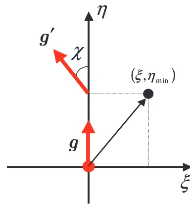
where the pairi and j satisfies Eq. (6), and we have ap-proximated that the impact parameter is given byb = ξi j in Eq. (4) as shown in Fig. 3. Thus, in the (ξ, η) coordinate system, the field particle position ξi j andηi j correspond to the velocity changeΔgi jand the time of the interaction
Δti j, respectively. This procedure will be repeated until the test particle leaves the prescribed interaction region, i.e. r<Δ/2 as depicted in Fig. 1.
Fig. 2 Algebraic trajectory (broken line) and exact trajectory (curved line) which is a part of a hyperbola. A field par-ticle (black circle) is on the left.
Fig. 3 Coordinate transform from the (x,y) to (ξ, η). In this co-ordinate system, the scattering angle χ, i.e. the impact parameterband the time of the interactionΔtare approx-imately given byξandη, respectively. The relative ve-locity att=0 isg, and isg=g+ Δgatt= Δt.
3. Calculation
The numerical results with using thedirect integration method, DIM, hereafter refers to that obtained by solving the following equation of motion a particle-iwith a charge qi, a massmi, and velocityuiat a positionri
mi dvi
dt =qi N
ji qj
4πε0 ri−rj
ri−rj
3. (9)
As the DIM in this study, we will use the 6-stage 5-th order Runge-Kutta-Fehlberg method known as the RKF65 [7, 8] with the absolute numerical error tolerance of 10−16.
Fig. 4 The typical initial conditions of particles; (a) positions normalized by the interparticle separation on the left, and (b) in the particle velocity normalized by the thermal speed on the right. The number of particles is 422.
interparticle separation,Δ. We will consider two cases: all the field particles are fixed at their initial positions, the Case 1, and moving field particles, the Case 2. The typical initial condition is depicted in Fig. 4. The numerical con-ditions correspond to a fusion plasma with a temperature ofT = 10 keV and a number density of n = 1020 m−3.
In such plasmas, the Debye length isλD ∼500Δ, where
Δ≡n−1/3.
3.1
Case 1: All field particles at rest
In the Case 1, all the field particles are at rest, and one of them locates at the origin. The test particle starts from the position of (b,−Δ/2) with a velocity of (0, v0). Thusb
is the impact parameter against the field particle initially at the origin.
Figure 5 is an example out of 105Monte Carlo calcu-lations for an impact parameterb =0.3Δ, and compares the algebraic (ALG) trajectory and the exact (DIM) tra-jectory normalized by the interparticle separationΔ. Note that the DIM results are accurate up to of the order of 10−16
which is the absolute error tolerance adopted. The circles in the figure indicate the positions at which the test parti-cle is given the impulse force by one of 441 field partiparti-cles. The algebraic (ALG) approximation agrees well with the direct integration method, DIM, in most cases as shown in Fig. 5.
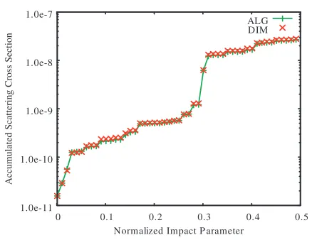
Depicted in Fig. 6 is theaccumulatedscattering cross sectionσacc(b) as a function of the impact parameterb
de-fined by
σacc(b)=
b
0
Δg g
2
πbdb
≈π(Δt)2 103
103b/Δ
k=1
k×Δgk2, (10)
whereΔgk
2
is the variance for the impact parameter bk=k×Δ/103with a Monte Carlo trials of 105adopted in this study. The agreement ofσALG
acc (b) with the exact one,
σDIM
acc (b), is also excellent. It should, however, be noted
that all the field particles are at rest throughout the calcu-lation in this case [5].
Fig. 5 Comparison of algebraic trajectory (denoted by ALG) and the exact trajectory (denoted by DIM, direct integra-tion method) in the case of two-dimensional 442-body Coulomb collisions with an impact parameterb=0.3Δ. Coordinates (x,y) are normalized by Δ. The circles in the figures for the algebraic trajectories stand for the po-sitions at which the test particle is given the impulse force by one of 441 field particles.
Fig. 6 Accumulated Coulomb scattering cross section normal-ized by the square of the average interparticle separation, σacc(b)/Δ2, vs normalized impact parameter ¯b=b/Δ
in the case ofN=442-body. See Ref. [5] for detail.
The two-dimensional total multibody scattering cross section forb=bmax= Δ/2 in Fig. 6 ,
σacc(bmax= Δ/2)∼2.8×10−8×Δ2, (11)
is more than 103times the conventional binary cross
sec-tion [9, 10],
σbin =4πb20ln
bmax
b0
∼2.3×10⁻¹¹×Δ2, (12)
with the maximum impact parameter bmax = Δ/2. As
test particle in the (x,y) plane that the interaction results in a large angle scattering in the 2-d calculation with, say, z=0, the same field particle locates not necessarily close to the test particle withz0 in 3-d.
The CPU time required for the algebraic approxi-mation is only about 20 min using a personal computer, whereas the exact analysis requires 15 hours to integrate the entire set of multibody equations of motion, i.e. the DIM.
3.2
Case 2: Moving field particles.
Strictly speaking, the Case 1 does not deal with the multibody problem, but solves the test particle motion in the presence of the multiple field particles at rest. In the Case 2, we will loosen the above restriction on the field particle motion, and have applied the algebraic model to the 442-body problem, in which there are 441 moving field particles and a test particle initially at rest. The two-dimensional 442-body system is analyzed for the time in-tervalΔt≡Δ/gth, i.e. the time for a particle with a thermal
speedgthto travel the interparticle separationΔ=n−1/3.
The change in positionΔr(results not shown) of the field particles during the time intervalΔtare in good agree-ment with the exact one, since they are moving in a very weak potential so thatΔri∼ui(0)Δtto a good approxima-tion. Although, the absolute value of the change in velocity |Δu|of each particle by the ALG are of the same order as the exact one, the orientation ofΔuis not correct as shown in Fig. 7, where the test particle starts at the upper-right point (U,V)=(0,0). Also depicted for reference in Fig. 7 is the final point att= Δtby using the BIA, the binary in-teraction approximation, proposed by the authors [6]. Note that the BIA accurately predicts the final point of the DIM with the absolute error tolerance of 10−16.
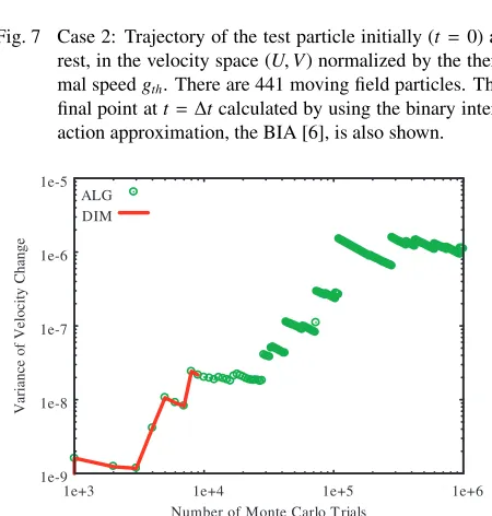
In spite of relatively poor accuracy in the individual particle motion, the ALG approximation still gives a good result for the statistical quantities, such as variance of ve-locity changes for a large number of Monte Carlo trials, NMC. The green circles in Fig. 8 for the ALG show the
variance of changes in normalized velocity,(Δu)2/g2 th, of
the test particle initially at rest as a function of the number of the Monte Carlo trialsNMC, in which the variance up to
NMC =104 with red line by using the DIM is also shown.
Several jumps seen in Fig. 8 are due to close encounters, i.e. large angle scatterings withΔvi/gth∼1. At the number
of Monte Carlo trialsNMC =104, the normalized variance
by using the ALG,(Δu)2 = 2.016×10⁻⁸×g2
th, agrees
with that due to the DIM,(Δu)2 = 2.022×10⁻⁸×g2 th,
within a relative error less than 0.3 %. As will be shown in Fig. 9 on the CPU times, the DIM forNMC = 106Monte
Carlo trials would need a CPU timeτCPU DIM ∼ 10
8 sec∼ 3
years, while only 2×10⁴sec∼6 hours for the ALG, both
on a personal computer (Intel Pentium 4, 2.60C GHz).
Fig. 7 Case 2: Trajectory of the test particle initially (t=0) at rest, in the velocity space (U,V) normalized by the ther-mal speedgth. There are 441 moving field particles. The
final point att= Δtcalculated by using the binary inter-action approximation, the BIA [6], is also shown.
Fig. 8 Variance of the change in velocity,(Δu)2/g2
th, of the test
particle initially at rest, in the case ofN=442-body; the Case 2. There are no data for the DIM beyond the Monte Carlo trialsNMC=104, since the DIM calculation needs
much time for largerNMC.
3.3
Comparison of CPU times
In the case of moving field particles as the Case 2, the CPU timeτCPUdependence on the number of particlesN= 442, 841, 1682, 3722, 10202, and 20450 is examined on the personal computer.
The red squares in Fig. 9 stand for the CPU time of the DIM with the red fitting line of
τCPU
DIM(N)∼2.06×10−
6×N2.83
sec. (13)
Note that the DIM forN=20450 was not examined since it would take a CPU time of the order of 37 days. The green triangles in Fig. 9 represent the ALG with the green fitting line of
τCPU
ALG(N)∼2.36×10−
10×N3.02
sec, (14)
and the blue circles for the BIA with the fitting line in blue,
τCPU
BIA ∼5.04×10−
6×N1.99
Fig. 9 CPU timeτCPU dependence on the number of particles
N = 442, 841, 1682, 3722, 10202, and 20450, on a typical PC (Intel Pentium 4, 2.60C GHz). Red squares stand for the CPU time for the DIM with a fitting line in red,τCPU
DIM∝N
2.83. Green triangles stand for the CPU time
for the ALG with a fitting line in green,τCPU ALG ∝ N
3.02.
Blue circles stand for the CPU time for the BIA with a fitting line in blue,τCPU
BIA ∝N 1.99.
(14), the ALG scheme calculates the variance of velocity changes 8.73×10³×N−0.19times as fast as the DIM, specif-ically the RKF65 method in this study. In other words, the ALG is faster than the DIM for the number of particleN less than 5.5×10²⁰. For a 108-body problem, which cor-responds to full three-dimensional Coulomb interactions within the Debye sphere in a fusion plasma, the ALG ap-proximation would still be 2.63×10²times as fast as the
DIM.
4. Conclusion
The algebraic model (ALG) proposed by the authors has sufficiently high accuracy in calculating the motion of a test particle with all the field particles at rest. When all the field particles are moving, however, the ALG has rela-tively poor prediction ability on the motion of the test parti-cle initially at rest. None the less, the ALG approximation gives good results for the statistical quantities, such as
vari-ance of velocity changes, i.e. the scattering cross section, for a sufficiently large number of Monte Carlo trials. The CPU time of the approximation is 8.73×10³×N−0.19times shorter than the 6-stage 5-th order Runge-Kutta-Fehlberg method with an absolute error tolerance of 10−16.
The numerical results presented here is for two dimen-sional systems with low density and high temperature, i.e. the small angle scatteringsχ 1, which is the most ap-propriate for the ALG as well as the BIA. We will soon apply the ALG/BIA to three dimensional cases, and/or to systems withχ∼1, such as the gravitationalN-body sys-tems, in the near future.
Acknowledgement
The authors would like to thank Dr. A. Wakasa, Prof. Y. Matsumoto and Prof. M. Itagaki for their fruitful dis-cussions on the subject. The author would also acknowl-edge the continuous encouragement of the late Prof. T. Yamashina. This research was partially supported by a Grant-in-Aid for Scientific Research (C), 21560061 from the Ministry of Education, Culture, Sports, Science and Technology (MEXT).
[1] A. W. Appel, SIAM J. Sci. Stat. Comput.6, 85 (1985). [2] J. E. Barnes and P. Hutt, Nature324, 446 (1986).
[3] P. P. Brieu, F. J. Summers and J. P. Ostriker, APJ453, 566 (1995).
[4] J. Makino and M. Taiji, APJ480, 432 (1997).
[5] S. Oikawa and H. Funasaka, Plasma Fusion Res.3, S1073 (2008).
[6] S. Oikawa, H. Funasaka, K. Higashi and Y. Kitagawa, Bi-nary Interaction Approximation to N-Body Problems, to be appeared in Plasma Fusion Res.4(2009).
[7] E. Fehlberg, NASA Technical Report 315 (1969).
[8] E. Fehlberg, Klassische Runge-Kutta-Formeln vierter und niedrigerer Ordnung mit Schrittweiten-Kontrolle und ihre Anwendung auf Warmeleitungsprobleme,Computing(Arch. Elektron. Rechnen), vol. 6, (1970) pp. 61–71.
[9] R. S. Cohen, L. Spitzer, Jr., and P. McR. Routly, Phys. Rev. 80, 230 (1950).