http://www.sciencepublishinggroup.com/j/ijass doi: 10.11648/j.ijass.20190701.12
ISSN: 2376-7014 (Print); ISSN: 2376-7022 (Online)
Temporal Variation of Ionospheric Scintillation in Relation
with Ionospheric Total Electron Content (TEC) over Ethiopia
Antneh Gashaye Tegegne
Department of Physics, College of Natural Science, Arba Minch University, Arba Minch, Ethiopia
Email address:
To cite this article:
Antneh Gashaye Tegegne. Temporal Variation of Ionospheric Scintillation in Relation with Ionospheric Total Electron Content (TEC) over Ethiopia. International Journal of Astrophysics and Space Science. Vol. 7, No. 1, 2019, pp. 12-20. doi: 10.11648/j.ijass.20190701.12
Received: June 27, 2019; Accepted: July 22, 2019; Published: August 6, 2019
Abstract:
In this study the amplitude scintillation intensity index (S4) and ionospheric total electron content (TEC) data of theyear 2012 obtained from Global Positioning System Scintillation Network and Decision (GPS-SCINDA) receiver wasanalyzed. The diurnal, monthly and seasonal variation of amplitude scintillation intensity index S4 and ionospheric total electron content
(TEC) observed from the analyzed data. It is found that intense scintillation occurred during the day time with a small frequency and very frequent occurrences of relatively moderate scintillation during the night time but the vertical total electron content weak at night time than day time. it is observed that ionospheric scintillation intensity index in March, April, February, September– December recorded scintillation events at moderate and intense levels, and these events were generally localized within 1930 LT–2400 LT and All other months experienced weak scintillation of various degrees of occurrences. The scintillation showed a seasonal variation characterized by intense values in March equinox compare to that of in June solstice season. The diurnal variations of amplitude scintillation intensity index S4 in relation with TEC showed that there is more
scintillation and TEC around 15:00 to 20:00 UT and this is may be due to the enhancement of equatorial spread F and formation of plasma bubble during the night.
Keywords:
Ionospheric Total Electron Content (TEC), Amplitude Scintillation Intensity Index (S4), Scintillation1. Introduction
Ionosphere is the ionized part of the Earth’s atmosphere which is formed primarily through the ionization of the atom and molecule in the upper atmosphere by ultraviolet (UV) radiation from the Sun. Recombination of electron and positive ions takes place continuously. The ionosphere is divided into D, E and F regions. Each layer is characterized by altitude range, composition and electron density concentration. The F region splits into F1 and F2 layer during the day. There is no solar radiation at night, however, the recombination takes place and so the D, E and F1 layer gradually diminish. After Sunset the F2 layer persists, although its density slowly decreases through the height. In terms of latitudes variation we can classify as low and equatorial, middle and high latitude ionosphere [1, 2].
The ionosphere is a highly dynamic medium characterized by irregularity. These irregularities are predominantly in the F layer of the ionosphere at altitude ranging from 200 to 1000 km, with the primary disturbance region being typically between
250 and 400km. It is well established that the large scale plasma depletion in the post Sunset period through the Rayleigh-Taylor instability and that the depleted region rise quickly to cover the entire F region including the topside ionosphere. Plasma depletions are the irregularities of the largest scale sizes (up to a few hundred km), where in the plasma density may be lowered by up to three orders of magnitude compared to the background plasma density, in relation to this there will be an enhancement of plasma density [3].
Ionospheric plasma density irregularities are an impediment to the radio wave communication as they result in scattering of the incident radio waves practically at all frequencies of interest. This phenomenon known as the ionospheric scintillations refers to the rapid fluctuations of the phase and amplitude of the radio wave signal. Which arise when a radio wave signal passes through the ionospheric region that is embedded with the plasma density irregularities [4].
produce scintillations in these two regions are quite different, leading to significant differences in the characteristics of the resulting scintillations. Auroral and polar cap scintillations are mainly the result of geomagnetic storms that are associated with solar flares and coronal holes. Unlike equatorial scintillations, they show little diurnal variation in their rate of occurrence, and can last from a few hours to many days, beginning at any time during the day [5]. Large and rapid variations in the plasma density are often associated with auroral and polar cap scintillations and can lead to significant errors in differential GPS (DGPS) systems as well as rapid changes in the apparent range and range rate [7, 8]. Auroral scintillations also show a seasonal dependence which is the reverse of that observed at low latitudes, being greatest from the autumn equinox through winter to the spring equinox, and a minimum during the summer months [7]. Indeed, the geomagnetic disturbances that excite auroral and polar cap scintillations tend to suppress the onset of equatorial scintillations during solar maximum periods [6, 8]. Because geomagnetic storm activity is linked to solar activity through solar flares and coronal holes, auroral and polar cap scintillations also show a strong dependence on the 11 year solar cycle, being most intense during solar maximum periods, but almost non-existent during minima.
Equatorial scintillations, on the other hand, are produced by irregularities in the F-layer of the equatorial ionosphere following the passage of the evening terminator and tend to disappear soon after midnight. In these regions, the most severe scintillations are associated with the crests of the equatorial anomaly which are centered approximately 15°either side of the magnetic equator [7]. As equatorial scintillations are coupled to the anomaly, they tend to be worse during the years of solar maximum when the anomaly is at its greatest.
Equatorial scintillations also show a strong seasonal dependence, being greatest during the months of April to August in the Pacific longitude sector, but a minimum during these months in the American, African and Indian sectors. This situation is reversed during the months of September to March [9]. During the seasons of high scintillation activity, the equinoctial months of March and September tend to suffer the highest levels of activity, although this does not appear to be true at all longitudes.
In this paper, only equatorial scintillations will be considered as they affect the largest number of people and tend to be more severe than their auroral counterparts [8]. In addition, the latitude band that is affected by equatorial scintillations covers approximately 50% of the Earth’s surface, compared to only 7% for the auroral and polar cap regions. However, it should be mentioned that during intense magnetic storms, auroral disturbances can extend well into the mid-latitudes, disrupting GPS through both scintillation activity and large density gradients. An example of this was the magnetic storm in March 1989 during which auroral scintillation effects were felt over most of the continental United States causing narrow bandwidth receivers to frequently lose signal lock [10]. Such events are, however, quite uncommon.
So, this studies aiming on investigation of the scintillation and TEC temporal variation. In doing so, the study discover the relationship between TEC and scintillation by observing diurnal, monthly and seasonal variation. Then after the total electron content in relation with amplitude scintillation intensity index S4 will be discussed.
2. Data Description and Analysis
2.1. Data Selection and Description
The data used in this analysis were collected with GPS ionospheric scintillation and TEC monitoring (GISTM) ground receiver originates from GISTM measurement using high data rate Novatel GSV400B GPS SCINDA dual frequency (L1=1575.42 MHz and L2=1227.60 MHz) receiver
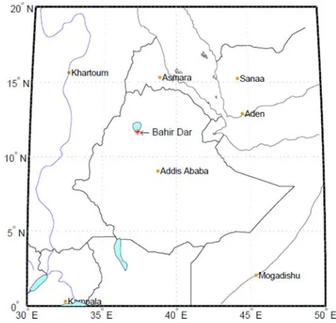
situated at Bahir Dar University, Bahir Dar, Ethiopia (11.3°N, 37.6°E) near-equatorial location in Africa (see Figure 1).
Figure 1. Map showing locations of scintillation receivers for Scintillation Network Decision Aid (SCINDA) sites at Bahir Dar.
Thus the observation data is stored in SCINDA format. This format consists of different ASCII file types. Each file type consists of a header section and a data section. Files stored in this format are generated by GPS-SCINDA software and differentiated according to their file name extension (*.xxx). Some file types that GPS- SCINDA can generate are ionospheric statistics (e.g S4, TEC, and ROTI) with extension
*
.scn, receiver position with extension *.psn, scintillation intensity data in the format used by SCINDA with extension *gps.dat and GPS raw observable (S/N ratios, pseudoranges and phases) with extension
*
.obs. But our parameter for this study are TEC and S4 among the
so called ionospheric statistics stored in the compressed files with the extension *.scn.
2.2. Method of Analysis
fluctuation in the amplitude and phase of Trans-ionospheric radio signal due to variation in the local index of refraction along the propagation path. GPS-SCINDA software measure the intensity of amplitude scintillation given by the scintillation intensity index S4 as;
S = 〈I 〉 − 〈I〉〈I〉
The SCINDA software uses the noise ratio converted to linear units as proxy for the signal intensity when computing the S4 index.
In this study, the analysis of the scintillation and TEC data has been carried out using the GPS TEC analysis application software called WinTEC-P, which was developed by Carrano and Groves (2009) at the Institute of Scientific Research, Boston College, USA. WinTEC-P is a Software written in C for the LINUX operating system which intended for the calibration of GPS TEC measurements made using GPS- SCINDA. It is an extension of a Kalman filter approach developed at NOAA/SEC for TEC calibration called WinTEC (MS Windows). The LINUX implementation includes estimation and removal of the plasmaspheric contribution to the TEC. The WinTEC-P software is distributed with GPS-SCINDA bundle and will be compiled automatically on the GPS-SCINDA data collection computer or on any computer running LINUX with the GNU R and GNU Scientific Library are installed. WinTEC- P utilizes the GPS-SCINDA ionospheric statistics file (*.scn) and the position file (*.psn) to obtain coordinates of the station, if it is not specified in its configuration [8].
The software includes an algorithm for the estimation and removal of instrumental biases associated with the GPS receiver and the GPS satellites. Depending on the options selected in the configuration, the WinTEC-P program can estimate the satellite biases from the data, or it can use satellite biases downloaded from CODE. The biases free TEC (Vertical TEC) and S4 index
are written in ASCII output files together with other parameter defining the position of the satellite such as the time, elevation angle, azimuth angle, and the longitude and latitude of the Ionospheric Pierce Points (IPP). It also includes programs write in the GNU R to plot S4 and calibrated TEC and Perl Scripts to
automatically generate a archive daily S4 and TEC plots with 15
minute updates.
Total Electron Content (TEC) from GPS: As we had discussed
earlier ionosphere is the region between 70-1000 km above the earth containing ionized gas and electrons. A wave traveling through it will experience a time delay. The radio signals from GPS on channels L1 (1575.42 MHz) and L2 (1227.6 MHz) will
experience difference delays [13, 14]. And it can be express mathematically as follow
∆t = 40.30TECcf , TEC = N (l) dl
TEC is a measure of the number of electrons along the path from the GPS satellite and is reported in TEC units (TECU = electrons1016 m−2).
The GPS-SCINDA software computes relative TEC (TECR)
as well as the differential pseudo-range and differential phase among other ionospheric statistics that can be used to obtain a more accurate TEC in post-processing. The relative TEC measurement computed by SCINDA software are based on 60 second averages of the differential pseudo-ranges (DPR) and differential carrier phase (DCP). The DPR is leveled to the DCP using all the data for each continuous phase arc.
TEC = DC P + (DP R − DC P)$ %
Once the relative TEC has been processed the calibrated TEC is obtained by subtraction of the satellite BS and receiver
BR differential code biases from the relative TEC as;
TEC = TEC − A(B − B )
Where A is a constant whose value is 2.854 TECU/ns. Using the single layer approximation for the ionosphere the calibrated slant TEC is converted to vertical TEC as follows;
TEC((B ) = )TEC − A(B − B ) * M(ε, h)⁄
Where M(ε, h) is the single layer mapping function of the ionosphere defined as:
M(ε, h) = sec 1sin45678cos :
78+ ℎ <=
Where Re is the Earth radius in km and ε is the elevation
angle in radians. Here h is the ionospheric height which is assumed at 350 km.
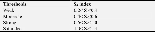
Using the GPS calibration software we were calibrate the GPS-SCINDA data. In order to study the level of scintillation we have chosen four distinct thresholds which are named as weak, moderate, strong and saturated given by Gwal et al., (2004) as tabulated below.
Table 1. Ionospheric amplitude scintillation thresholds.
Thresholds S4 index
Weak 0.2< S4≤0.4
Moderate 0.4< S4≤0.6
Strong 0.6< S4≤1.0
Saturated 1.0< S4≤1.4
Based on the above chosen distinct threshold we have discussed the diurnal, monthly and seasonal variation of ionospheric amplitude scintillation index S4 with total electron
content (TEC).
3. Result and Discussion
3.1. Introduction
In this study the ionospheric amplitude scintillation intensity index S4 and the vertical total electron content data of the year
2012 obtained from Global Positioning System Scintillation Network and Decision (GPS-SCINDA) dual frequency (L1=1575.42 MHz and L2=1227.60 MHz) receiver situated at
scintillation intensity index S4 in relation with vertical total
electron content.
3.2. Diurnal Variation
The diurnal variation of S4 from January to December
2012 is shown in the figure 2. So, the S4 value ranges from
0.02 to 1.14. Particularly, the smallest values are observed from 0200 to 2000 in almost the cases. The relatively high
values are observed from 2000 to 0200 and ranged from 0.08 to 0.14. This general trend confirms the fact that the scintillation is significant during the night. However, it can be seen from figure 2 that small amount of intense scintillation occurred during the day time. The result generally exhibit an occurrence frequency of scintillation observed mainly at nighttime hours (2000-0000 extended to 0200 LT in some cases).
Figure 2. Diurnal variation of S4 from January to December 2012.
The diurnal variation of vertical total electron content (VTEC) is shown in the figure 3. The plot indicates that the minimum value is near sunrise, then TEC increase until
maximum value is around 1400-1500 L T, after that decrease through the night. It also indicates that the VTEC value range from 5 to 45.
Figure 3. Diurnal variation of vTEC from January to December 2012.
3.3. Monthly Variation
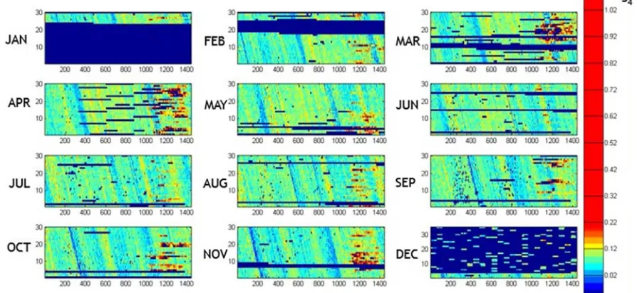
The monthly variation of scintillation intensity index S4 is
discussed as shown in figure 4. In all the plots, larger
February, September– December recorded scintillation events at moderate and intense levels, and these events were generally localized within 1930LT–2400LT, although, the distributions
were observed to extend to around 0300LT during January, February and December. All other months experienced weak scintillation of various degrees of occurrences.
Figure 4. Monthly variation of the scintillation index S4.
The monthly variation of ionospheric total electron content (VTEC) is shown in the figure 5 The diurnal variation shows that vTEC variation depends on the solar zenithal angle. vTEC values are lower than 20 TECU from midnight to 1100 and from 1700 to midnight. The highest values are observed
during the course of the day and particularly around 1500 LT where we have values greater than 20 TECU. The highest values are observed in the months of March, October and September.
Figure 5. Monthly variation of the vTEC.
3.4. Seasonal Variation
Figures 6 to 11 show respectively the seasonal variation of the scintillation index S4 and vertical total electron content
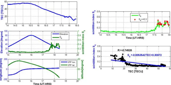
(vTEC) in March equinoxes and June Solstices. In March equinox, from figures 6 to 8 panel one shows the vertical total electron content (vTEC) as we have seen from this panel vTEC does not show significant variation from 11:00 to
17:00 UT, but immediately from 17:00 to 24:00 UT fluctuation in vTEC is observed. In panel four of this Figure the scintillation intensity index S4 does not shown significant difference from 11:00 to 17:00 UT and the value of S4 is less
than 0.2, but after 17:00 UT when fluctuation in vTEC is observed the scintillation intensity index S4 shoots up with
Figure 6. Variation on vertical TEC and S4 index of March equinox.
Figure 7. Variation on vertical TEC and S4 index of March equinox.
In June solstice, from figures 9 to 11 the vertical total electron content (vTEC) as shown in panel one of the Figures does not show significant variation or the variation is linear throughout the time. In relation to that panel four of this figure
depicts something about amplitude scintillation intensity index S4. That is, as we have seen in the Figure the scintillation
intensity index S4 does not have a value greater than 0.2
throughout the time, so it is insignificant.
Figure 9. Variation on vertical TEC and S4 index of June solstice.
Figure 10. Variation on vertical TEC and S4 index of June solstice.
Finally, we can say that the fluctuation of total electron content and variation of the scintillation is appreciable at night. It is more significant in equinoxes than in solstices with a higher rate of occurrence in March equinox, and it may be due to the Sun is overhead at the equator during equinox season.
4. Conclusions
The study started by calibrating GPS-SINDA data of year 2012 on a station located a Bahir Dar University, Ethiopia. Then after by analyzing the calibrated data we observe the diurnal, monthly and seasonal variation of ionospheric scintillation intensity index S4 and vertical total electron
content (TECv) of the equatorial ionosphere. Thus the following conclusions can be drawn from the results obtained:
The result showed that the diurnal variation of amplitude scintillation intensity index S4 has intense value during the
day time with a small frequency and relatively moderate scintillation occurrence during the night time with very frequent occurrence of scintillation. Whereas the vertical total electron content (VTEC) has a maximum value during the day time after sunset the TEC value decreases. This may be due to the dependency on the solar zenithal angle and night time phenomena of equatorial ionosphere such as plasma bubble formation and equatorial spread F which leads to irregularity in the region. When we goes through the monthly variation of ionospheric scintillation intensity index March, April, February, September– December recorded scintillation events at moderate and intense levels, and these events were generally localized within 1930LT–2400LT and All other months experienced weak scintillation of various degrees of occurrences. Beside our results have demonstrated that on seasonal variation, the amplitude scintillation intensity index S4 shows that significantly enhances and peak occurs in
March equinox than that of June solstice. This depicts that scintillation occurrence is high in March equinox season.
Generally, in our location we have frequent occurrence of weak ionospheric scintillations, while few intense scintillations. Scintillations are normally more frequent, due to generation of equatorial irregularities and the irregularities suppressed by magnetic disturbance.
Acknowledgements
I would like to thank Washera Geospace and Radar Science Laboratory, Bahir Dar University, Bahir Dar, Ethiopia for the availability of GPS-SCINDA data.
References
[1] Emirant Bertillas Amabayo, Multi-instrument observations of ionosphericirreg-ularities over South Africa, Masters thesis, 2011.
[2] J. K. Hargreaves, R. D. Hunsucker, The high-latitude ionosphere and its effects on radio propagation, p. 244-249. [3] Schunk, R. W. and A. F. Nagy, Ionospheres, Physics, Plasma
physics and Chem- istry. Cambridge, Atmospheric and Space science series, 2005.
[4] J. O. Olwendo, P. J. Cilliers, P. Baki, C. Mito, Using GPS-SCINDA observations to study the correlation between scintillation, total electron content enhancement and depletions over the Kenyan region, Advances in Space Research vol 49, 2012.
[5] Klobuchar, J. A., Global Positioning System: Theory and Applications, Volume I, Progress in Astronautics and Aeronautics, vol. 163, Chapter 12, pp. 485-515, 1996. [6] Klobuchar, J. A., Ionospheric Effects on GPS, GPS World, pp.
48-51, April 1991. Koleva R. Sauvaud J. -A., Plasmas in the near Earth magnetotail lobes: Properties and sources, J. Atmos. Terr. Phys., pp. - 2118-2131. - Vol. 70, 2008.
[7] Aarons, J. A., Equatorial Scintillations: A Review, IEEE Transactions on Antennas and Propagation, vol. AP-25, No. 5, pp. 729-736, 1977.
[8] Anita Aikio and Tuomo Nygren, 761658 S IONOSPHERIC PHYSICS, Department of Physical Sciences, University of Oulu, 2008.
[9] C. E. Valladaras, J. Villalobos, R. Sheehan and M. P. Hagan, Latitudinal exten- sion of low-latitude scintillations measured with a network of GPS receivers, Ann. Geophysicae, vol. 22, pp. 3155-3175, 2004.
[10] Maruyama, T. Ionosphere and Thermosphere. Journal of the Communications Research Laboratory, 49 (3): 163-179, 2002. [11] Paschmann G., Haerendel G., Sckopke N. Rosenbauer H.,
Plasma and Magnetic Field Characteristics of the Distant Polar Cusp Near Local Noon: The Entry Layer, J. Geophys. Res., pp. - 16: Vol. 81, 1976.
[12] Piddington J. H., Twists and rotations of solar magnetic fields, Astrophysics and Space Science, p. 273-287: Vol. 75, 1980. [13] Pr¨olsGerd W. Physics of the Earth’s Space Environment An
Introduction. - Berlin Heidelberg: Springer, 2004.
[14] Richardson John D., PaularenaKarolen I., Lazarus Alan J. Belcher John W., Radial evolution of the solar wind from IMP 8 to Voyager 2, Geophys. Res. Lett., p. 325-328. - 4: Vol. 22, 1995.
[15] A. Gil, M. V. Alania, Advances in Space Research 45 (2010) 429436.
[16] A. Gil, R. Modzelewska, M. V. Alania, ACTA PHYSICA POLONICA B Vol. 39 (2008) No 5.
[17] Kenneth Davies, Ionospheric Radio, Peter Peregrinus Ltd, United Kingdum, May 1989.
[18] http://www.ngdc.noaa.gov/ngdc.html, December 3, 2011. [19] D. K. Sharma, J. Rai1, M. Israil, P. Subrahmanyam, P. Chopra,
and S. C. Garg, Annales Geophysicae (2004) 22: 20472052 SRef-ID: 1432-0576/ag/2004-22-2047
[21] Sheeley N. R., Walters J. H,, Wang Y. M. Howard R. A., Continous tracking of coronal outflows: Two kinds of coronal mass ejections, J. Geophys. Res. -Space Physics, p. 24739-24767. - A11: Vol. 104, 1999.
[22] Suvorova A. V., Dimitriev A. V. Kuznetsov S. N., Dayside magnetosphere mod- els, Radiation Measurements, pp. - 687-692. - 5: Vol. 30, 1999.
[23] Swarzschild M., On noise arising from the solar granulation, Astrophys. J., p. - 1: Vol. 107, 1948.
[24] Robert W. Schunk and Andrew F. Nagy, IONOSPHERES, Physics, Plasma Physics, and Chemistry, Second Edition, 2000 (2009).
[25] Song Y. Lysak R. L., Some Theoretical Aspects of the Solar Wind- Magneto- spheric Interaction, Phys. Chem. Earth, pp. - 715-721. - 7-8: Vol. 22, 1997.
[26] Levine R. H., Altschuler M. D. Harvey J. W., Solar ources of the Interplanetary Magnetic Field and Solar Wind, J. Geophys. Res., p. - 7: Vol. 82, 1977 b.
[27] Levine R. H., Altschuler M. D., Harvey J. W. Jackson B. V., Open Magnetic Structures On The Sun, Astrophys. J., p. 636-651. Vol. 215, 1977 a.