Study of Magnetic Island Using a 3D MHD Equilibrium Calculation Code

Study of Magnetic Island Using a 3D MHD Equilibrium

Calculation Code

∗

)

Yasuhiro SUZUKI

_{, Satoru SAKAKIBARA}

_{, Kiyomasa WATANABE}

_,

Yoshiro NARUSHIMA

_{, Satoshi OHDACHI}

_{, Satoshi YAMAMOTO}

_,

Hiroyuki OKADA

_{and LHD experiment group}

1)_{National Institute for Fusion Science, Toki 509-5292, Japan}

2)_{Graduate University for Advanced Studies (SOKENDAI), Toki 509-5292, Japan}

3)_{Institute of Advanced Energy, Kyoto University, Uji 611-0011, Japan}

(Received 13 February 2011/Accepted 31 May 2011)

Coupling the magnetic diagnostics and a 3D MHD equilibrium calculation code, the magnetic island is studied in the Large Helical Device (LHD) experiment. In an experiment, the collapse in the plasma core was observed in a configuration, which has large magnetic island produced by external perturbation coils. At the collapse, the temperatur profile was flattened. This suggests the magnetic island evolved. The magnetic island was observed by the magnetic diagnostics. The magnetic diagnostics also suggests evolving the magnetic island. A 3D MHD equilibrium is caluclated by the 3D MHD equilibrium code then signals of the magnetic diagnostics are simulated. Since the comparison of observed and calculated signals is comparable, the magnetic island in calculated equilibrium is similar to one of the experiment.

c

2011 The Japan Society of Plasma Science and Nuclear Fusion Research

Keywords: magnetic island, MHD equilibrium, magnetic diagnostics, HINT2, JDIA DOI: 10.1585/pfr.6.2402134

1. Introduction

The study of the magnetic island is an important is-sue because the generation of the magnetic island leads the degradation of the confinement due to flattering of the tem-perature. In tokamaks, the magnetic island is generated by the resistive MHD instability like the tearing mode [1] at many cases. Especially, the study of the neoclassical tear-ing mode (NTM) [2] is an important and critical issue. On the other hand, in stellarator/heliotron plasmas, the gener-ation of the magnetic island is observed due to the MHD instability [3,4]. In addition, the evolution and suppression of the magnetic island are also observed without the MHD instability [5]. In such cases, the magnetic island is driven by the equilibrium response [6–8]. Since the magnetic is-land driven by the equilibrium response is not rotating and appeared in the quasi steady-state, it is good target to mea-sure the magnetic island.

To observe the magnetic island, the profile measure-ment is widely used. Flattening of the electron temperature and density indicate the existence of the magnetic island. However, if the O-point of magnetic islands does not lo-cate on the line of sight, the profile measurement cannot identify the magnetic island. On the other hand, the mag-netic diagnostics directly observe the plasma response and it does not depend on the location of the O-point. The mag-netic diagnostics observes total plasma response in the out-author’s e-mail: [email protected]

∗)_{This article is based on the presentation at the 20th International Toki}

Conference (ITC20).

side of the plasma. Thus, to identify modes of the plasma response, the mode analysis is done. In the LHD experi-ments, the mode analysis assuming the current filament is used [9] but this analysis can not model the magnetic field structure. To model the magnetic field more physically, coupling with the numerical simulation is necessary.

An advantage of the LHD device to study the mag-netic island is superposing of the resonant perturbation field (RMP) by external coils. These coils are called to the LID coils, which were prepared for the operation of the Lo-cal Island Divertor (LID) [10]. Since these coils can gener-ate the low-nmagnetic island for the vacuum, we can study only the effect of the plasma response on the magnetic is-land. Many experiments were done to study the plasma response [5, 11–13]. In those studies, the spontaneous evo-lution and suppression of the island were observed without the MHD instability. This suggests a possibility the mag-netic island changes spontaneously due to the equilibrium response. This also suggests 3D MHD equilibrium analy-sis can be used to study the magnetic island.

In this study, we study the magnetic island in a low magnetic shear configuration in the LHD. We propose studies of the magnetic island by coupling the magnetic diagnostics and a 3D MHD equilibrium calculation code without assumption of nested flux surfaces. In the next section, we show an experimental result, which is an obser-vation of the perturbation driven by the plasma response. The perturbed field is observed by the magnetic

diagnos-c

2011 The Japan Society of Plasma

tics. In Sec. 3, we show a demonstration of our method by coupling the magnetic diagnostics and the 3D MHD equi-librium code. Finally, we discuss and conclude this study.

2. Experimental Results

The LHD is anL/M=2/10 heliotron. HereLandM are the pole number of helical coil winding and toroidal field period. In this study, we did an experiment withn/m

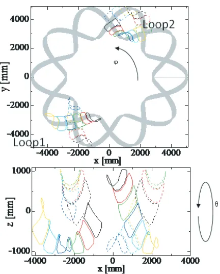
= 1/1 magnetic island, where n andm are toroidal and poloidal mode numbers, respectively. As mentioned in the introduction, the LHD device can produce low-nmagnetic islands by the LID coils. The LID coils produce the dipole field to producen/m = 1/1 field. The plasma response on low-n magnetic islands is observed by the magnetic diagnostics, which are two poloidal arrays of flux loops, “Loop1” and “Loop2”. Figure 1 shows a schematic view of poloidal arrays of flux loops. One array consists of twelve flux loops. These arrays measure the perturbed field pro-duce by the parallel current j. In the LHD experiments, jis the Pfirsh-Schl¨uter (P-S) current. If there is no low-n perturbed field smaller than the toroidal field period, two arrays observe same signals. However, appearing low-n perturbation (n <10), the difference between two arrays appears. From the difference, we can decide the perturbed fieldBr, mode numbersn/mand phase of the magnetic is-landφisland.

Figure 2 shows a discharge in a large plasma aspect ratio configuration (Ap = 8.3). In this experiments, the

Fig. 1 The schematic view of poloidal arrays of flux loops. Two arrays are installed atφ=57 and 237 [deg]. One array consists of twelve loops.

dipole field by LID coils was superposed to a configura-tion, which isRax=3.6 m andκ ∼1. TheRaxis the

vac-uum axis position andκis the averaged elongation of the plasma. The dipole field resonates onι=1 surface, where ι is the rotational transform. The order of the perturbed fieldB11is aboutO(10−4). The width of the island is about Δρ∼0.4, whereρis the normalized minor radius. ForAp =8.3 configuration, the rotational transform on the axisι0

is larger thann/m=2/3 and the rotational transform at the plasma edge onιais smaller thann/m=3/2. This means

onlyn/m=1/1 island appears in this configuration and it can be considered. The magnetic shear onι=1 surface is weaker than other configurations with smallAp. Thus, we

can expect the equilibrium response will appear strongly. In the figure, the volume averaged betaβdia, the plasma

current Ip/Bt, signals Φr at a poloidal angle and the

dif-ferenceΔΦr between two arrays at the poloidal angle are

plotted. A red line indicates the time appearing the mi-nor collapse. IncreasingΔΦr,βdiaslightly decreases. In

Fig. 3, profiles of the electron temperatureTebetween the

Fig. 2 The volume averaged beta βdia, the plasma current

Ip/Bt, signalsΦr at a poloidal angle and the difference

ΔΦrbetween two arrays at the poloidal angle are plotted. The minor collapse apperas at the red line in the figure.

Fig. 4 Measured flux from two poloidal arrays are shown be-tween the collapset=0.65 and 0.86 [s]. Profiles are plot-ted along the poloidal angleθ. Differences between Loop 1 and 2 are increased after the collapse.

collapse are plotted. After the collapse,Tedecreases then

flatteningTeincreases. This suggests the magnetic island

withn/m=1/1 evolves.

In Fig. 4, profiles of measured flux on loop arrays are plotted along the poloidal angleθ. Profiles are shown at t=0.7 (before the collapse) and 0.86 (after the collapse). After the collapse, the difference increases and signals of the Loop1 is sensitive. Although the signal of the Loop2 is almost same at different times, the signal of the Loop1 changes. This means the perturbation of the plasma re-sponse is large under the Loop1.

In this experiment, we observe magnetic fluctuations by magnetic probes. However, the low-nMHD instability to produce the magnetic island was not observed strongly. Thus, the perturbed field may be produced by the equilib-rium response.

3. Comparison of Magnetic

Diagnos-tics and a 3D MHD Equilibrium

In this section, we study a 3D MHD equilibrium

cal-culation and it is compared with the magnetic diagnostics. The magnetic diagnostics observes the perturbation of the plasma response from the outside of the plasma. Ob-served signals are total perturbations and its depend on the internal distribution of the plasma current density. Thus, to understand the magnetic field structure, other analyses are necessary. A method is the mode analysis assuming currents filaments in the plasma. In this method, the multi-filament currents If = Imncos(mθ−nφ+α) are put on the resonant surface, where Imn andαare the maximum filament current and the phase of the mode, respectively. Symbolsθandφshow poloidal and toroidal angles on the Boozer coordinate system. The subscriptsm andn indi-cate the poloidal and toroidal mode numbers. The spatial structure of the mode is identified through the compari-son between observed perturbation and the calculated flux. From these procedures, we can identify the mode and ap-proximated location of the plasma response. Details are shown in ref. [9]. However, in this analysis, the magnetic field structure cannot be identified because filament cur-rents are assumed. If we can get the internal distribution of the plasma current density jplasma, we can reconstruct

the external perturbation from the internal jplasma

distribu-tion. A candidate to get jplasma is the information from

the 3D MHD equilibrium calculation if the magnetic is-land is changed by the equilibrium response. The 3D MHD equilibrium calculation gives the information of the mag-netic field (jplasma). The DIAGNO [14], V3FIT [15] and

JDIA [16] codes were developed to couple a 3D MHD equilibrium code, VMEC [17]. Using those codes, we can compare observed signals and calculated perturbation without the magnetic island because the VMEC assumes perfectly nested flux surfaces. This means those code can-not identify the magnetic island breaking nested flux sur-faces. To identify the magnetic island, coupling the JDIA and HINT2 codes was proposed. The HINT2 is a 3D MHD equilibrium calculation code without assumptions of per-fectly nested flux surfaces [18].

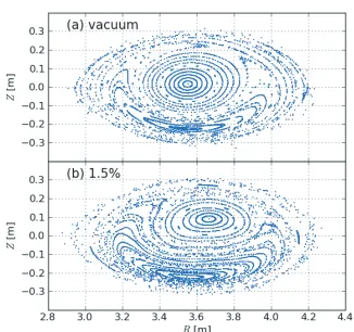
In Fig. 5, flux surfaces including n = 1 island are shown for the vacuum and a finite-βequilibrium. The cal-culation was done forRax =3.6 m,Ap =8.3,κ ∼1

cor-responding to the experiment. These cross sections are same at the poloidal section along the Thomson scatter-ing system (the chord is along onZ = 0 const. plane). The equilibrium calculation was done with the initial pres-sure profilep = p0(1−s)(1−s4), whichsis the

Fig. 5 Poincar´e plots of magnetic field lines withn/m = 1/1 island are shown for the vacuum field and a finite-β equi-librium (β ∼ 1.5%). The configuration is an inward shifted configuration (Rax = 3.6 m, Ap = 8.3, κ ≈ 1). The color-bar indicates the connection length of magnetic field lines.

Fig. 6 Calculated flux on poloidal loop arrays are plotted corre-sponding to Fig. 4.

field. The nonlinear coupling of those modes leads the stochastization of field lines.

Figure 6 shows calculated flux of poloidal loop arrays from HINT2 and JDIA corresponding to Fig. 4. The order of the flux between the calculation and observation is com-parable but the factor is different. The profile is similar in both cases. Especially, the Loop1 is sensitive in the cal-culation and it corresponds to the experiment. From this calculation, we can guess the magnetic field structure from Fig. 5. In Fig. 3, the temperature collapse was observed but that was not the collapse. According to Fig. 5,n/m= 1/1 island evolved then the magnetic axis shifted upward. Therefore, the electron temperature was observed on the O-point of the magnetic island.

4. Discussion and Summary

We proposed the study of the magnetic island by cou-pling the magnetic diagnostics and the HINT2 code. Ob-served and calculated flux on poloidal loop arrays are com-parable then the magnetic island evolves due to the

equi-librium response. However, the difference is found in the comparison. The order of the flux is same but the factor is a little bit different. In this study, we compare with only one calculated equilibrium assuming a pressure profile and zero net toroidal current. Since the poloidal loop array is sensitive to the pressure profile, we need to compare with other equilibria with different pressure profiles.

The net toroidal current is observed. Here, we dis-cussed only the equilibrium response due to the distortion of the P-S current flow. If the magnetic island appears or changes, the distortion of the net toroidal currents, which are the Ohmic, beam-driven and bootstrap currents as ex-amples, along the magnetic island is not surprising. As an example, a theory predicted the evolution and suppres-sion of the magnetic island by the bootstrap current [19]. The consideration is analogy from the theory of the NTM. In tokamaks, the bootstrap current always destabilizes the tearing mode. However, in stellarator/heliotron, the mag-netic shear is the reversed shear in tokamaks. Thus, the bootstrap current will suppress the magnetic island. For the real plasma in the experiment, the equilibrium response is coupled the effect of the P-S and other currents nonlin-early because the spontaneous evolution and suppression of the island can not be explained by only the P-S current in the experiment [5]. In that change, the magnetic island spontaneously changes due to the plasma collisionality in a discharge. To understand the equilibrium response includ-ing othe currents, the extension of the HINT2 code is nec-essary. The HINT2 can treat only the net-toroidal current prescribed by the function of the toroidal flux. In this treat-ment, the vanishing of the bootstrap current in the island cannot be represented. The extension is now doing. In-cluding the neoclassical current self-consistently, the cou-pling the HINT and transport codes is necessary. That is a future subject.

Achkonwledgements

This work is performed with the support and under the auspices of the NIFS Collaborative Re-search Program NIFS07KOAP018, NIFS10KUHL037 and NIFS10KTAT047. This work was supported by Grant-in-aid for Scientific Research for Young Scientists (B) 20760585 from the Ministry of Education, culture, Sports, Science and Technology.

[1] H.P. Furthet al., Phys. Fluids16, 1054 (1973). [2] Z. Changet al., Phys. Rev. Lett.74, 4633 (1995). [3] S. Sakakibaraet al., Fusion Sci. Technol.50, 177 (2006). [4] S. Sakakibaraet al., Fusion Sci. Technol.58, 176 (2010). [5] Y. Narushimaet al., Nucl. Fusion48, 075010 (2008). [6] A.H. Reiman and A.H. Boozer, Phys. Fluids 27, 2446

(1984).

[7] J.R. Cary and M. Kotschenreuther, Phys. Fluids28, 1392 (1985).

[9] S. Sakakibaraet al., Fusion Sci. Technol.58, 471 (2010). [10] N. Ohyabuet al., J. Nucl. Mater.266, 302 (1999). [11] K. Nariharaet al., Phys. Rev Lett.87, 135002 (2001). [12] N. Ohyabuet al., Phys. Rev Lett.88, 055005 (2002). [13] N. Ohyabuet al., Plasma Phys. Control. Fusion47, 1431

(2005).

[14] H.J. Gardner, Nucl. Fusion30, 1417 (1990).

[15] S.P. Hirshmanet al., Phys. Plasmas11, 595 (2004). [16] T. Yamaguchiet al., Plasma Fusion Res.1, 011-1 (2006). [17] S.P. Hirshman et al., Comput. Phys. Commun. 43, 143

(1986).

[18] Y. Suzukiet al., Nucl. Fusion46, L19 (2006).