http://www.sciencepublishinggroup.com/j/ijdst doi: 10.11648/j.ijdst.20170302.12
ISSN: 2472-2200 (Print); ISSN: 2472-2235 (Online)
Intelligence Classification of the Timetable Problem: A
Memetic Approach
Eboka Andrew Okonji, Yerokun Mary Oluwatoyin, Okoba Ifeoma Patricia
Department of Computer Education, Federal College of Education Technical, Asaba, Nigeria
Email address:
[email protected] (E. A. Okonji), [email protected] (Y. M. Oluwatoyin), [email protected] (O. I. Patricia)
To cite this article:
Eboka Andrew Okonji, Yerokun Mary Oluwatoyin, Okoba Ifeoma Patricia. Intelligence Classification of the Timetable Problem: A Memetic Approach. International Journal on Data Science and Technology. Vol. 3, No. 2, 2017, pp. 24-33. doi: 10.11648/j.ijdst.20170302.12 Received: April 5, 2017; Accepted: May 15, 2017; Published: July 27, 2017
Abstract:
Scheduling tasks persist in our daily functioning and as academia, abounds more in University circle as hard-NP constraint satisfaction tasks. Many studies exist with the objective of resolving the many conflicted constraints that exists in a timetable schedule using various algorithms. Many of such algorithms simply search the domain space for a goal state that satisfies the problem constraints. Our study yields an outcome assignment that provides a complete, feasible and optimal academic schedule that satisfies medium cum hard constraints for the Federal University of Petroleum Resource Effurun in Delta State of Nigeria using memetic algorithm. Results showed that model converges after 4minutes and 29seconds; while its convergence time depends on use of belief space to ensure agents do not violate model bounds, encoding scheme used amongst others. The schedule considers both instructors and students’ preference as medium constraints of high priority.Keywords:
Fitness, Constraints, Cross-Over, Mutation, Timetable, Memetic Algorithm, Intelligent, Schedule1. Introduction
University timetable is a continuously evolving study that is often plagued by conflict resolution whose careful management and planning is of the essence – in order to yield a feasible schedule that is friendly to both instructors and students. The field of problem solving aims at resolving such issues that continue to bedevil the management of timetable in the Nigerian University (case in point). The case often – is that reports have shown, Government has no prerequisite funding to provide adequate infrastructure and the needed laboratories that will help to improve the quality of education. These and other constraints, continues to hamper effective management and planning of timetable (as well as examination, as the crux of the education system and certifies that awardees have been found worthy in character and learning as bestowed with the responsibility deserving of the certificate an awardee possess (NEEDs Report, 2015). Survey inspections via the Committee for Budget Monitoring setup on the Federal Government of Nigeria / Academic Staff Union of Universities (FGN/ASUU) 2009 memoranda of understanding, posits that this problem is far from being resolved in nearest time possible as government perceives education as a money-gulping (rather than money-yielding
sector of the nation). This, Government insists on their terms has necessitated the downward review of monetary allocation as clearly seen from the Federal Government’s 2016 Budgetary Allocation – for which 8-percent of the total allocation goes to fund the educational sector (2016 Budget). This makes the examination timetable planning purely, a constraint satisfaction task (ASUU, 2015).
Constraint satisfaction problem (CSP) consists of 3-parts: (a) variables, (b) values satisfying each variable, and (c) set of constraints that makes possible assignment of a value to each variable. Thus, the task aims at a domain that seeks solution to a set of problem via a search algorithm or model that assigns values to each variable with the aim of satisfying each variable as well as adhering to all possible constraints (Zhang and Lau, 2005; Ozcan, 2005; Ojugo et al, 2016). Every assignment is a state in a search space. An assignment of values to all variable is termed complete; partial if some variables are not satisfied with values, and an assignment is
consistent if it violates not constraints that help assign an optimal value to its variable (Coddington, 2012; Ojugo et al, 2015, 2016).
approximate-feasible, optimal and complete solution: given a set of instructors, assigned a corresponding set of lectures classes (courses) for timeslots within certain days of the week, such that with a corresponding set of enrolled students, the task results in a tuple scheduled event for Ni
instructor-class pair within Nt timeslots to yield a schedule where no
instructor or student is in more than one lecture class at a time, and no room is expected to accommodate more than its capacity and more than a lecture at a time (Abrahamson et al, 1996; Anh et al, 2006; Miners et al, 1995; Saleh Elmohamed et al, 1998; Kumal and Dowd, 2005; Michaelwicz, 1998; Ojugo et al, 2016).
A. Constraints Types in Timetable Problem (TTP)
Constraints are divided into (Saleh Elmohammed et al, 1998; Ojugo et al, 2007; 2016) thus:
a. Hard constraints are specific to room-time conflicts. They cannot be physically violated or overlapped as such event constraints must be satisfied. We can schedule only one examination per class per time for an instructor, student or room as thus: (a) courses taught by the same instructor, (b) examination of courses that were taught in same room, (c) lectures or labs of the same class, (d) courses cannot be assigned to a particular room unless the room capacity is greater or equal to number of student enrollment for same class, and (e) laboratory courses or classes require a certain type of room.
b.Medium constraints are all instructors/students
preference that are based on room-time conflict that also cannot be physically violated (e.g. a student cannot be in more than one class at the same time). However, it is not possible to as a rule of thumb to always satisfy all students. Thus, we aim to avoid via adjustments so that though we are not expected to satisfy all student-lecture preferences – in some cases, students can adjust their preferences to satisfy student-lecture preference if such course class conflicts or is oversubscribed. Some students will carry-over certain courses, and these must be taken into account. Medium constraints do not have costs as high as hard constraints attached to them; But, it is aimed seriously that in a final schedule, such cost(s) or penalty must be minimized and preferably, reduced to zero where possible. Examples are: (a) avoid timeslot conflicts for lectures with students in common, (b) eligibility criteria for the class must be met, and (c) do not enroll athletes in classes that conflict with their sport practice time, etc.
c. Soft constraints are preferences of time conflicts, and they have lowest penalty associated to them. Example include: (a) for each student level, have a fully-packed 3-days of the week (Mondays, Wednesdays and Fridays) and less-packed 2-days (Tuesdays and Thursdays), (b) spread time lectures over the entire week, (c) lecture classes may involve contiguous time, (d) balance student enrollment in multi-section lecture classes, (e) breaks may be specified, (f) instructor may request periods in which their lectures and classes are
not taught, (g) instructors have preference for specific rooms or types of rooms, and (h) minimize distance between room where classes are taught or assigned and the building housing the home department.
Thus, we aim at an event schedule of classes to instructors and their ranks with rooms assigned based on students enrollment and their preferences of which lecture or class to attend (when and their engagement in other activities during other timeslots), room capacity or size, class types and locations, distances between buildings where these rooms are located, priorities of each building as used by different departments, amongst other constraints. Thus, our objective is to constructs a feasible, optimal and complete schedule for students, taken by instructors that satisfies all hard constraints, and minimizes all soft and medium constraints (Brailsford et al, 1998; Saleh Elmohammed et al, 1998; Zhang and Lau, 2005; Michalewicz, 1998; Ojugo et al, 2016).
This implies that all hard constraints must be satisfied and their corresponding associated cost should be eliminated; while our medium and soft constraints (involving instructors’ and students’ preferences) should be satisfied where possible, or can be minimized such that the cost associated with them is brought to its minimum (though – preferences involving instructors takes precedence and higher priority over those of students). A feasible, optimal schedule is one that satisfies all hard constraints, minimizes all medium and soft constraints where they are not satisfied (Ojugo et al, 2016). The study was conducted via a semi-automated prediction. Its cost function measures quality of the current schedule that involves the weighted sum of penalties associated with the different constraint or violation types. The study thus, aims to find the optimal solution using stochastic, evolutionary methods that minimizes the cost function (Miners et al, 1995).
B. Related Literature on TTP
Ojugo et al (2016) employed simulated annealing algorithm with 3-heating strategy (with reheating, adaptive cooling and exponential cooling methods) for academic scheduling at the University of Benin, and adopted a rule-based preprocessor model to yield initial solutions. Their results showed that SA with exponential cooling proved best with solution converging after 2.112seconds, and that convergence of SA is dependent on parameters like start population, initial/ final temperature as well as random swaps applied in the cooling strategies. While the model offers great insight into the task at hand, it does not provide us with the ability to discern from the experimentation if the results compares better to other methods. Also, there is no means of storing the schedules so that model can backtrack its previous schedules and pick the best for the semester at any single time.
genetic algorithm and compared their results against standard genetic algorithm performance in generating possible timetables schedule. In their quest for better convergence of an optimal solution, their results of the modified GA used to schedule 2013/2014 rain semester exam at Ladoke Akintola University of Technology, Ogbomoso, Nigeria with a task involving 19,127students, 200-courses, 53-venues and 2-weeks (excluding Saturdays and Sundays) outperforms standard GA and maintains its accuracy level with increase in problem size; whereas standard GA lost its effectiveness as the problem size grows. While, their work provides useful insight into further investigation of TTP, we observe these: (a) their study had no sample output schedule, (b) did not account for course-room-time conflict (if schedule yields complete assignment of instructors to courses with venues and timeslots with no conflicts) – then there will be no need for study as classes have rooms appropriately allocated to them, (c) instructor preferences out-weights those of student and was not also accounted for, (d) instructors have ranks that must be catered for as senior ranked instructors are often times engaged in administrative duties, (e) challenges with adjunct instructors was not accounted for, (f) though, study considered only examination – distance between venues for students with concurrent examination was not accounted, and (h) their study initially set out to simulate and store results generated in each iteration so that they can easily detect conflicts via results, the best schedule over time (this goal was not achieved).
C. Statement of Problem
1.Seek further insight into the field of problem solving in Computer Science, exchange idea in the domain as well as further equip policymakers with adequate useful data required for such scheduling. Thus, we employ statistical stochastic models and heuristics as in Section II/III.
2.As a non-Euclidean, complex, chaotic, dynamic, highly
multi-dimensioned and multi-objective task with its range of applications as a scheduling task makes it
critical as a determinant in many activities that resonates a University system. Supervised schedules are time-wasting and often redundant, yielding inconclusive cum unsatisfying result and lots of copy and paste work
– with many unresolved
instructor-student_enrollment_room_size conflicts as well as swaps in instructor/student preference amongst others. This leads to increased ‘unresolved’ non-complete and non-optimal schedules. To curb this, see Section III.
3.Such studies are often hampered by such ever-evolving
feats like instructors ranks/preferences, student
enrollment and preferences, distances between
buildings, class type and capacity etc – yielding the unavailability of a precise and concise datasets as its dataset is often littered with ambiguities, noise and partial truth. This must be resolved via a robust search method as in Section III.
4.Resolution of speed defects that often traps hill-climbing method at local maxima as used by
evolutionary models is here resolved via hybridization of statistical methods as in Section III as no one method yields better solution than hybrids. These hybrids, also in turn impose conflicts of statistical dependency from dataset used and from the idea of merging heuristics. This is resolved via discretization of model and data encoding as in Section III, which will also help model avoid overtraining, over parameterization and over-fitting.
D. Objective of Study and Rationale
The goal is: (a) implement a genetic algorithm trained fuzzy neural network model, (b) ensure model is statistically sound to simulate such complex, chaotic and dynamic event, and lastly, (c) compare its statistics/result to those of other hybrids, using the same dataset.
Rationale for this choice is that for evolutionary models, no single heuristics is as good as hybrids. The case in point being that the genetic algorithm trained fuzzy neural network model will simply have the following benefits:
1.The fuzzy set provides the initial solution for the model to perform its simulation and prediction.
2.We employ the Jordan neural network constructed from
a multi-layered perceptron network with
Backpropagation and momentum-in-time learning rate that allows network to store output progress and use same output as feedback into the system to create another generation of schedule.
3.Model exploits GA’s speed to ensure that the model is never trapped at local maxima.
4.Model implores GA’s flexibility and exploratory ability to seek at each generation, a global maxima or optimal (best schedule) is found as each generation forms the backdrop for a better (schedule) pool. And, in turn, makes model more robust and can be easily tuned.
2. Proposed Model Framework /
Methodology
Soft computing is an inexact science that seeks to propagate observed data, as the model seeks the underlying probabilities of data feats of interest to yield an expected output, chosen from a set of possible solution space and is guaranteed of high quality even with noise, ambiguity and impartial truth applied at its input. It exploits numeric data to perform quantitative processing via a search algorithm that explores solution space and ensures qualitative knowledge as output, and experience as its new language (Ojugo et al, 2013). Our hybrid model hinges on 4-methods: (a) fuzzy logic, (b) genetic algorithm, (c) artificial neural network and (d) decision support system.
A. Fuzzy Logic System
Fuzzy system chooses between different control actions and transforms them into a fuzzy set value, (Nascimento, 1991; Ludmila, 2008; Ojugo et al, 2016) which is divided into:
on an object’s description, so that it can predict each class label. Object descriptions are vector values with attributes relevant for classification task. Classifier learns to predict a class labels via training algorithm and its accompanying dataset. If training data is not available, the classifier is designed to learn apriori so that when trained, it classifies data focusing on If-Then rules with actions and outcomes, constructed as a user specifies class rules and linguistic variables (fuzzy set) that helps tune a fuzzy set in line with such class rules (Ludmila, 2008).
b.Fuzzy Cluster groups data as linguistic variables into homogeneous classes known as clusters so that items in the same class are as similar as possible, and vice-versa (Yang and Wang 2001). Based on data and task, it uses different measures to identify classes and to control how
clusters are formed. Such measures include
connectivity, distance and intensity (Ojugo et al, 2012). In some cases (non-fuzzy/hard clusters), data is divided into clusters so that each data point belongs to exactly one cluster; But, in fuzzy clusters, a data can belong to more than one cluster. Each data is associated with member-grades that indicate degree to which a data point belongs to different clusters.
Linguistic variable(s) helps to convey data about a task or data under observation (Inan and Elif, 2005). They can overlap to share feats about other data under observations also. In this study, it is used to indicate distance between rooms where lectures occur and buildings in department – via the term far. We all may have slightly different ideas about the exact distance that far represents even when this distance is consistent (Berks et al 2000). Some students may agree it is not far and at some point, they also agree that it is far. The space between far and not far indicates distance to some degree, which is actually a bit of both. Thus, the horizontal axis measures the value of distance; while, its vertical axis measures the degree to which the linguistic variable fits the measured data (Inan and Elif, 2005; Ojugo et al, 2016).
To represent linguistic variable(s), we use fuzzy cluster mean that attempts to partition a finite set of elements into a set of clusters in relation to given criterion (Berks et al 2000; Ojugo et al, 2016) by computing arithmetic means of all data. See Ojugo et al (2016) for FCM algorithm and the adopted fuzzy logic system performance tuning.
We adopt the fuzzy model by Ojugo et al (2015) – which yields a recursive heuristic that assigns an event of time_space to lecture-class_student-enrollment slots suited to the problem domain. Also, the model’s basics function has the data files of lecture-classes, room_space/buildings, department_buildings, distance_matrix, student_enrollment and inclusion data. Thus, using these structures – the system builds an internal database used to perform the scheduling. Its internal processes are such that checks distances between buildings, room_space_type and time allotted, and compares cum resolves all room_space and time_slot conflicts. It also tracks and updates hours already scheduled. Thus: scheduling is done by department, so that each move is generated as loop
over all the departments. The departments are chosen in order of size, with those having the most classes or lectures being scheduled first. The model first scans all currently unscheduled lectures. It then attempts to assign them to the first unoccupied rooms and timeslots that satisfy the rules governing constraints. Constraints for room capacity is difficult to satisfy, larger classes are scheduled first to result iteration and speed of processing as well as avoid conflicts in room exhaustion (Ojugo et al, 2015).
In most cases, only rooms and timeslots satisfying all rules will already by occupied by previously schedule; And in such case, the system attempts to move a lecture/class into a room and timeslot and allow the unscheduled lecture class to be scheduled. Next, system searches the schedule to select those with higher cost by checking all medium and soft constraints (e.g. how close a room match a class-size, how many students have lecture-time conflicts or clashes, which sporting activity conflicts with lecture-time, the student enrollment affected, if a lecture is in a preferred timeslot, room or building, and so on). If a poorly scheduled lecture class is identified, the model searches the space, maps or swaps it into a more comfortable timeslot – so that the hard constraint are still satisfied, but the overall cost of medium/soft constraints are reduced. Room swapping process continues, provided all the rules are satisfied and no cycling (swapping of the same lecture) occurs. Once all the departments have been schedule, iteration cycle is complete. The model continues until complete iteration yields no further change in a schedule. There are many rules dealing with room_time conflict, room type, room_priority etc – many of which are complex. Our fuzzy model yields partial schedule as output (though, it is unable to assign all the given classes to room_time slots). Output is grouped into: list of unassigned classes from constraint conflict, and list of all assigned cum associated instructors/student_enrollment to room_time. The basic rules for implementing these constraints include (Ojugo et al, 2015):
a. IF room_size > student_enrollment AND {no conflict in room} THEN ASSIGN Room to the Lecture-Class. b.IF Instructor = (Professor > Adjunct > Reader > Senior
Lecturer > LecturerI > LecturerII) AND {NO room_time conflict} THEN (allot room to most senior instructor as preference).
c. IF (Time = allotted lecture) AND Student_has_Sports THEN Adjust Student OR Class_Time.
Our fuzzy model will yield a partial schedule as output (as it is unable to assign all the given lectures to rooms and timeslots). Output is grouped these: (a) list of unassigned lecture classes from constraint conflict, and (b) classes and all the associated instructors/students_enrolled_set as assigned to various rooms [26,39,41].
B. Artificial Neural Network (ANN)
connections (Caudill, 1987 and Fausett, 1994). As learning takes place, model adjust its node weights and biases as well as converts the data so that depending on the task, it uses an activation/transfer function to modulate the associated input (Mandic and Chambers, 2001) and nonlinear feats exhibited in the task to yield an output via Eq. 1. Its weights are correlated as Wi.j which sums all weights between input and hidden layers, Woj is the bias and xi is TTP input data. Thus, it yields an output via the tangent/sigmoid function that sums its weighted input as in Eq. 2 and Eq. 3 (Minns, 1998; Chakraborty, 2010).
∅ = = ∑ ∗ (1)
= + ∑ ∗ (2)
= !∗"#$− 1 (3)
There are 2-types of ANN: feedforward and recurrent. For this study, we use recurrent (Jordan) network with
unsupervised learning (Ojugo et al, 2016). The Jordan net is constructed by adding a context layer to (modify) a multilayered feedforward and using a backpropagation-momentum-in-time unsupervised learning to train the data. This will help it retain data between iterations. As algorithm starts, the context layer is initialized to 0, so that output from the first iteration is fed back as input into its hidden layer (Perez and Marwala, 2011; Ojugo et al, 2016). Thus, in next time step, previous contents of the hidden layer is processed to yield an output, which is also resent into context layer as new input (and repassed as input into hidden layer in another time-step to yield output). Process continues till solution is found (Regianni and Rientjes, 2005). Weights are recomputed in same manner for new connections fro/to its
context layer from hidden layer. Training aims at best fit data weights computed via Tansig function that assumes an approximation influence of data points at its center.
'( = + ∑ )*- (∗ ∅ + , = + ∑- *(∗ ∅||' − / || (4)
Arriving at best schedule (optimal solution) requires previous knowledge. So, model incorporates previous data and model previous output (fed back as input) into hidden units (Rajurkar et al, 2004; Karunanthis et al, 1994) to yield another output. Our model (net) resolves the structural
dependencies imposed by dataset and by the hybrid
heuristics used through its ability to store earlier data generated from previous layer(s) (Kuan, 1994; Ojugo et al, 2016) and through the encoding decimal encoding used in the GA. Feedforward nets can be expanded and extended to represent complex dynamic patterns such as this – since, it treats all data as new so that previous data do not help to identify data feats, even if such observed datasets exhibits temporal dependence; But, as the network grows larger, it becomes practical difficult. However, Jordan net overcomes this difficulty through these internal feedbacks, and the Jordan net is more plausible and computationally more powerful than other adaptive models.
Its learning algorithm allows output at time t to be used alongside new input to compute another output at time t+1 in response to dynamism. Thus, first output is fed-back as input to hidden layers with a time delay, so that outputs at time t−1
is input at time t (Mandic and Chambers, 2001) computed by its activation function yk in Eq. 4, which sums input, receives target value of input training pattern, computes error data, weight correction updates in layers (cjk) and bias weights
correction updates (cok). The errors are sent from output layer
back to input nodes via backpropagation (which helps correct the weights and to find weights that approximate target output with selected accuracy). Weights are modified by minimizing error between target and computed outputs; And, if the error is higher than selected value, process continues – else, training stops with weights updated via mean square error until model achieve minimal error (Ursem et al, 2002; Ojugo et al, 2016).
C. Genetic Algorithm (GA)
GA is inspired by survival of fittest evolution and consists of population (data) chosen for selection with potential solutions to a specific task. Each potential solution is an individual for which optimal is found using four operators: initialize, select, crossover and mutation (Coello et al, 2004 and Reynolds, 1994). Individuals with genes close to optimal, is said to be fit. Fitness function determines how close an individual is to optimal solution. Ojugo et al (2013a,b) GA operators include: (a) initialize (encodes input data into a suitable form, uses fitness function to evaluate how close each solution is to its optimal so that they can be selected for mating if found to be good. The fitness function has knowledge of task and if more solutions are found, the higher its fitness value, (b) selection pick solutions that meets fitness criteria and ensures the fittest are chosen for mating on first come basis; Since, if waits to select only best fit after process ends, model may end up with an elitist solution, which often leads to local optima or poor convergence), (c)
crossover ensures best fit individual genes are exchanged to yield a new, fitter pool via a (1-, 2- or multi-point) cross with genes of a parent), and (d) mutation (helps to alter or introduce greater diversity or chaos to ensure that the new pool yields the best or converges to global minima, and the algorithm stops if optimal is found, or after number of runs if new pools are created).
possible individuals GA generates till an optimum is found (Reynolds, 2004).
3. Experimental Model
A. Experimental Model Framework
We adoptOjugo et al (2015) model proposed in the study as:
a. Knowledgebase of historic, decimal encoded data
(feats) and database of data matrix of TTP using fuzzy If-Then rules represented as linguistic variables with optimized membership functions. The fuzzy set consists
classifier to propagate if-then rule values of selected data, enhanced as predefined linguistic variables and classified into TTP classes. It uses the fuzzy cluster means universe discourse equation to enhances linguistic variables partitioned into data-point.
b.Inference Engine consists of our genetic algorithm trained neural network model. It infers conclusion derived from selected data encoded as fuzzy rules to yield a centralized, fuzzy function boundary in determining high/low degree membership function. We use Jordan net to provide self-learning optimized via crossover and mutation with an aim to re-introduce greater diversity and chaos that will help resolve all
conflicts to autonomous-scheduled events.
c.Decision support consists of the predicted output and the output database that is updated automatically in time as patients are diagnoses as long as it encounters and read sin new data. The decision support predicts system output based on the cognitive and the emotional filers as display by the output device.
Model starts off with Proposed Fuzzy Classifier and Cluster Mean Universe Discourse Equation (PFCMUDE) as in Eq. 6 to generate a fuzzy Linguistic variable Universe of discourse:
0 12345 = ∑ 6, 8, 1 … ∗ 0 (6)
A, B, C… = selected questions option; P(x) = probability assigned to questions option fuzzy range value.
Model starts off with Proposed Fuzzy Classifier and Cluster Mean Universe Discourse Equation (PFCMUDE) as in Eq. 6 to generate a fuzzy Linguistic variable Universe of discourse:
0 12345 = ∑ 6, 8, 1 … ∗ 0 (7)
A, B, C… = selected questions option; P(x) = probability assigned to questions option fuzzy range value.
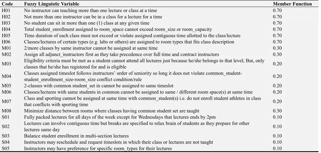
Table 1. Fuzzy Encoded Universe of Discourse for TTP.
Code Fuzzy Linguistic Variable Member Function
H01 No instructor can teaching more than one lecture or class at a time 0.70
H02 Not more than one instructor can be in a class for a lecture for a time 0.70
H03 No student can sit in more than one (1) class at any given time 0.70
H04 Total student_enrollment assigned to room_space cannot exceed room_size or room_capacity 0.70
H05 Time duration of each class must not exceed or violate assigned contiguous time allotted to the class/lecture 0.70 H06 Classes/lectures of certain types (e.g. labs or others) are assigned to room types that fits class description 0.70
M01 2/more classes by same instructor cannot be assigned at same time 0.30
M02 Assign all adjunct_instructors first as they take precedence over full time and contract instructors 0.30
M03 Eligibility criteria must be met as a student cannot attend all lectures just because he/she belongs to that level; But, only
classes that he/she has registered for and is eligible 0.20
M04 Classes assigned timeslot follows instructors’ order of seniority so long it does not violate
common_student-student_enrollment_size-room_size conflict condition/rule 0.20
M05 2-classes with common student_set in cannot be assigned to same timeslot 0.20
M06 Classes/lectures with same students in common cannot be assigned to same / different room space(s) at same time 0.20
M07 Class and sporting cannot be assigned at same time with common_student(s) i.e. do not enroll student athletes in class
that conflicts with sporting time 0.20
M08 Minimize distance between rooms where classes having common student set are taught 0.30
S01 Fully packed lectures for all days of the week except for Wednesdays that lectures ends by 2pm 0.10
S02 Lectures can involve contiguous time but breaks are specified to relax brain of students as they prepare for other
lectures same day 0.10
S03 Balance student enrollment in multi-section lectures 0.10
S04 Instructors may reschedule and request timeslots in which their class or lectures are not taught 0.10
S05 Instructors may have preference for specific room_types for their lectures 0.10
B. Genetic Algorithm Trained Neural Network (GANN)
GANN is initialized with 30-individuals rules whose fitness is computed and new pool is selected via tournament
method, which determines individual solutions selected for mating. We apply a multi-point crossover to help net learn all dynamic and non-linear feats in dataset (feats of interest). We then apply mutation, to add further diversity and reintroduce chaos so that best fit schedules are chosen. Data are randomly generated via Gaussian distribution corresponding
low fitness to yield new pool. Process continues until individual with a fitness value of 0 is found – indicating that the solution has been reached (Branke, 2001).
Initialization/selection via ANN ensures that first 3-beliefs are met; mutation ensures fourth belief is met. Its influence function influences how many mutations take place, and the knowledge of solution (how close its solution is) has direct impact on how algorithm is processed. Algorithm stops when best individual has fitness of 0 (Campolo et al, 1999; Dawson and Wilby 2001b). Ojugo et al (2016) CGA belief rules are:
a. Normative belief – each instructor and students is bound to only a class/lecture as a time given by 0.5).
b.Domain – events occurs daily from 8am-5pm, excluding Saturday and Sundays. It lists all department building and room_types to be allotted, and student_enrollment.
c. Temporal – is data structure of instructors (adjuncts) enrolled for both semester detailing each semester feats, student_enrollment for each lecture and those for sports. d.Spatial – creates the data structure of instructors enrolled, student enrollment for each lecture, buildings and their distances, rooms allocation and distances between all the rooms in various building, laboratory, pavilions etc
e. Influence function mediates between belief space and the pool – to ensure and alter individuals in the pool to conform to belief space.
GANN model is as thus: INPUT:
1. Pool_ size (k), crossover (c), mutation (v), influence function (Ic) and n; // Initialization and Selection
2. Randomly generate K possible solution
3. Save solution in population Kok; // Loop till terminal point
4. For m = 1 to n do; // Crossover
5. Number of crossover nc = (k – Ifnc)/2; 6. For u = 1 to n do;
7. Select two solutions randomly EA and FG for K;
8. Generate GV and HN by multi-point crossover to EA
and FG;
9. Save GV and HN to K2;
10.End For; //Mutation
11.For u = 1 to n do;
12.Selection a solution Yh from K2;
13.Mutate each bit of Yh under Ifnc
14.Generate a new solution Yhi
15.If Yhi is impossible
16.Recompute Yhi with possible solution by modifying Yhi
17.End if
18.Recompute Yhwith Yhi in K2
19.End for //Recompute
20.Recompute K = K2;
21.Return Best solution in Y
Model stops if stop criterion is met. GANN utilizes number of epochs to determine stop criterion. Initial selection (solution) that yields the 2nd generation is given as:
1. R1: If H01 Then C1 = 0.50
2. R2: If H01 & H02 Then C2 = 0.50 3. R3: If H01, H02 & H03 Then C3 = 0.50 4. R4: If H01, H02, H03 & H04 Then C4 = 0.50 5. R5: If H01, H02, H03, H04 & H05 Then C5 = 0.50 6. R6: If H01, H02, H03, H04, H05 & H06 Then C6 =
0.50
7. R7: If C6 & M01 Then C7 = 0.40
8. R8: If C6, MO1 & M02 Then C8 = 0.37
9. R9: If C6, MO1, MO2 & M03 Then C9 = 0.33
10.R10: If C6, MO1, MO2, MO3 & M04 Then C10 = 0.30
11.R11: If C6, MO1, MO2, MO3, MO4 & M05 Then C11
= 0.30
12.R12: If C6, MO1, MO2, MO3, MO4, MO5 & M06 Then C12 = 0.30
13.R13: If C6, MO1, MO2, MO3, MO4, MO5, MO6 & M07 Then C13 = 0.29
14.R14: If C6, MO1, MO2, MO3, MO4, MO5, MO6,
MO7 & M08 Then C14 = 0.30
15.R15: If C6, C14 & S01 Then C15 = 0.30 16.R16: If C6, C14, SO1 & S02 Then C16 = 0.25 17.R17: If C6, C14, SO1, SO2 & S03 Then C17 = 0.22 18.R18: If C6, C14, SO1, SO2, SO3 & S04 Then C18 =
0.22
19.R19: If C6, C14, SO1, SO2, SO3, SO4 & S05 Then C19 = 0.21
Fitness function (f) is resolved with initial pool (Parents) as:
R1:50 R2:50 R3:50 R4:50 R5:50 R6:50
R7:40 R8:37 R9:33 R10:30 R11:30 R12:30
R13:29 R14:30 R15:30 R16:25 R17:22 R18:22
R19:21
Fitness function (f) is resolved with first pool (dual Parents):
R1:53 R2:51 R3:48 R4:29 R5:55 R6:53
R7:31 R8:19 R9:25 R10:18 R11:40 R12:17
R13:54 R14:38 R15:45 R16:42 R17:39 R18:28
R19:32
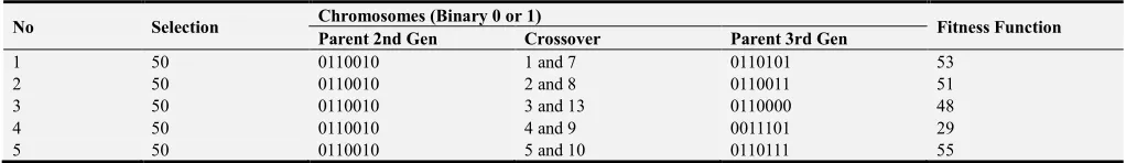
Table 2. 1st and 2nd Generation of population from Parents.
No Selection Chromosomes (Binary 0 or 1) Fitness Function
Parent 2nd Gen Crossover Parent 3rd Gen
1 50 0110010 1 and 7 0110101 53
2 50 0110010 2 and 8 0110011 51
3 50 0110010 3 and 13 0110000 48
4 50 0110010 4 and 9 0011101 29
No Selection Chromosomes (Binary 0 or 1) Fitness Function
Parent 2nd Gen Crossover Parent 3rd Gen
6 50 0110010 6 and 11 0110101 53
7 40 0101000 7 and 12 0011111 31
8 37 0100101 8 and 16 0010011 19
9 33 0100001 9 and 17 0011010 26
10 30 0011110 10 and 19 0010010 18
11 30 0011110 11 and 14 0110010 40
12 30 0011110 12 and 15 0010001 17
13 29 0011101 13 and 16 0110110 54
14 30 0011110 Mutation 0110000 38
15 30 0011110 15 and 19 0101101 45
16 25 0011001 Mutation 0101010 42
17 22 0010110 Mutation 0101001 39
18 22 0010110 18 and 2 0011100 28
19 21 0010101 19 and 1 0100000 32
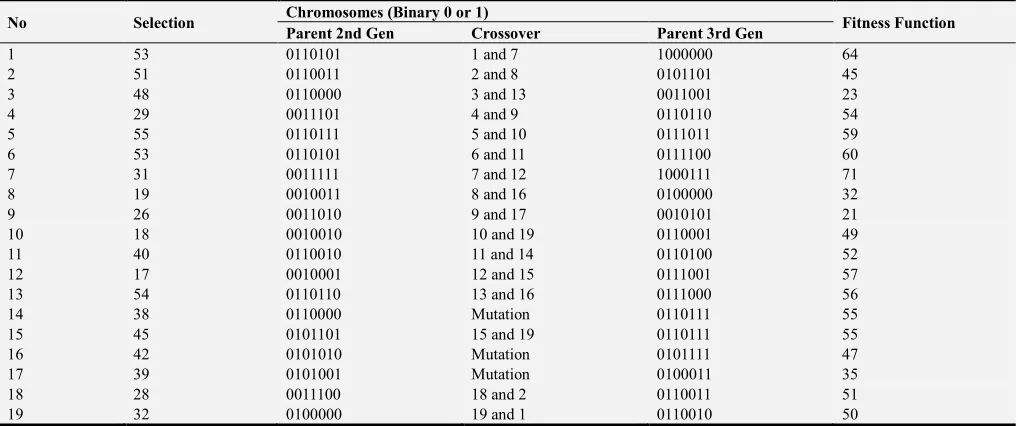
Table 3. 3rd and 4th Generation of population from Parents.
No Selection Chromosomes (Binary 0 or 1) Fitness Function
Parent 2nd Gen Crossover Parent 3rd Gen
1 53 0110101 1 and 7 1000000 64
2 51 0110011 2 and 8 0101101 45
3 48 0110000 3 and 13 0011001 23
4 29 0011101 4 and 9 0110110 54
5 55 0110111 5 and 10 0111011 59
6 53 0110101 6 and 11 0111100 60
7 31 0011111 7 and 12 1000111 71
8 19 0010011 8 and 16 0100000 32
9 26 0011010 9 and 17 0010101 21
10 18 0010010 10 and 19 0110001 49
11 40 0110010 11 and 14 0110100 52
12 17 0010001 12 and 15 0111001 57
13 54 0110110 13 and 16 0111000 56
14 38 0110000 Mutation 0110111 55
15 45 0101101 15 and 19 0110111 55
16 42 0101010 Mutation 0101111 47
17 39 0101001 Mutation 0100011 35
18 28 0011100 18 and 2 0110011 51
19 32 0100000 19 and 1 0110010 50
Tables 2 and 3 shows generation of optimized fuzzy linguistic variables of both single and dual parents by choosing first and second bits from the left as our crossover and mutation points. Third generation is our stop criterion with best fitness function of 71 (row 7) – implies that clusters of the various universe of discourse variable values as searched, has been optimized to 0.71 (with base value 0.50). Thus, if parameter combination yields a membership function less than 0.50, it is said to be a low-degree membership; while, those ≥ 0.50 is said to be high-degree membership function. It was also discovered that the more crossover and mutation is applied to the fuzzy linguistic variable as in tables 2 and table 3 respectively, the better and higher fitness function is reached by each solution. Thus, event scheduling accuracy increases as more time-steps are given allowing for better scheduling and random swaps.
4. Result Findings and Discussion
A schedule yields an assignment that satisfies the following:
1. R1: IF schedule satisfies only one hard constraint, without resolving any medium cum soft constraints;
THEN we classify such assignment as C1, which is non optimal and incomplete.
2. R2: IF schedule satisfies two hard constraints, without any medium cum soft constraints resolved; THEN we classify such assignment as C2, which is non optimal and incomplete.
3. R3: IF schedule satisfies three hard constraints, without any medium cum soft constraints resolved; THEN we classify such assignment as C3, which is non optimal and incomplete.
4. R4: IF schedule satisfies four hard constraints, without any medium cum soft constraints resolved; THEN we classify such assignment as C4, which is non optimal and incomplete.
5. R5: IF schedule satisfies five hard constraints, without any medium cum soft constraints resolved; THEN we classify such assignment as C5, which is non optimal and incomplete.
other medium and soft constraints. Thus, it is optimal but incomplete since we seek a solution that
eliminates all hard constraints as well as
minimize/eliminate all medium cum soft constraints. 7. R7: IF schedule satisfies all six hard constraints and a
medium constraint, without satisfying all medium and soft constraints; THEN we classify such assignment as C7, which is optimal but incomplete.
8. R8: IF schedule satisfies all six hard constraints and two medium constraints, without satisfying all medium and soft constraints; THEN we classify such assignment as C8, which is optimal but incomplete. 9. R9: IF schedule satisfies all six hard constraints and
three medium constraints, without satisfying all medium and soft constraints; THEN we classify such assignment as C9, which is optimal but incomplete. 10.R10: IF schedule satisfies all six hard constraints and
four medium constraints, without satisfying all medium and soft constraints; THEN we classify such assignment as C10, which is optimal but incomplete. 11.R11: IF schedule satisfies all six hard constraints and
five medium constraints, without satisfying all medium and soft constraints; THEN we classify such assignment as C11, which is optimal but incomplete. 12.R12: IF schedule satisfies all six hard constraints and
six medium constraints, without satisfying all medium and soft constraints; THEN we classify such assignment as C12, which is optimal but incomplete. 13.R13: IF schedule satisfies all six hard and seven
medium constraints, without satisfying any soft constraints; THEN we classify such assignment as C13, which is optimal but incomplete.
14.R14: IF schedule satisfies all six hard and seven medium constraints, and a soft constraint – without satisfying all soft constraints; THEN we classify such assignment as C14, which is optimal but incomplete. 15.R15: IF schedule satisfies all six hard and seven
medium constraints, and two soft constraint – without satisfying all soft constraints; THEN we classify such assignment as C15, which is optimal but incomplete. 16.R16: IF schedule satisfies all six hard and seven
medium constraints, and three soft constraint – without satisfying all soft constraints; THEN we classify such assignment as C16, which is optimal but incomplete. 17.R17: IF schedule satisfies all six hard and seven
medium constraints, and four soft constraint – without satisfying all soft constraints; THEN we classify such assignment as C17, which is optimal but incomplete. 18.R18: IF schedule satisfies all six hard and seven
medium constraints, and five soft constraint – without satisfying all soft constraints; THEN we classify such assignment as C14, which is optimal but incomplete. 19.R19: IF schedule satisfies all six hard, all seven
medium and all six soft constraints; THEN we classify such assignment as C19, which is optimal and complete.
After training and testing the model, results indicate that
the model took 4minutes and 29seconds to find optimal solution after 298-iterations (at best). The model was also ran 25 times (to eradicate non-biasness) and each time, it found optima – though convergence time varied from one epoch to another. It was observed that the convergence time depends on:
a. How close the initial population is to the solution b.Use of the belief spaces that ensured that each candidate
solution had upper and lower bounds that they could not violate. This, ensured solutions were never trapped at
either local maxima (ridges) or global minima
(plateau).
c. The initial encoding of the dataset used by the GA (here we adopted the binary encoding) – which though resulted in greater diversity of the solution space, it made easier the capability of the model to perform its processing more effectively.
d.Number of mutation applied to solutions in the pool. e. Our solution (search) space was made even closer via
our use of the fuzzy variable dataset (as a preprocessor).
5. Conclusion and Recommendations
While hybrid have been noted as being ever more tedious to implement than single heuristics – due to: (a) the statistical dependencies imposed on it by individual adopted methods, and (b) the conflicts to be resolved that are imposed on it by the dataset used. Here, we resolved such dependencies and conflicts via: (a) proper encoding scheme used to represent the dataset, (b) effective parameter selection, (c) proper modeling of the hybrid heuristic (like our choice of ANN model suitable for the task at hand) and using GA to speed up its capability, (d) our selection method (tournament) that allowed the best candidate solution to be selected into the pool at any time, and (e) use of structured learning. These feats also help modeler to avoid overtraining, over-fitting and over parameterization in such a multi-agent populated and multi-objective task.
Also, proper encoding of dataset allows the model to explore all candidate solutions more effectively by exploiting historic data in search of an optimal solution – because as agents force their own behavioral rules on dataset, the belief space of the model helps to curb their influence – so that the model becomes the new language for the agents. Thus, models must serve as vehicle to convey knowledge and to advance investigation into more complex, chaotic and dynamic events.
References
[1] Academic Staff Union of Universities (2015). Downward review of the monetary allocation in defiance of FGN/ASUU 2009 MOU, Gaurdian Newspaper, Wed 18 November, 2015, pp 32 – 33.
[3] Chakraborty, R., (2010). Soft computing and fuzzy logic, Lecture notes, retrieved from
http://www.myreaders.info/07_fuzzy_systems.pdf.
[4] Delamaire, L and Abdou, H., (2009). Credit card fraud and detection techniques: a review, Banks and Bank Systems, 4(2), pp57.
[5] Heppner, H and Grenander, U., (1990). Stochastic non-linear model for coordinated bird flocks, In Krasner, S (Ed.), The ubiquity of chaos pp.233–238. Washington: AAAS.
[6] Kennedy, C and Porter, A., (2013). Fraud detection and prevention, [online]: retrieved July 2015 from www.moss-adam.com/fraud_reviews.
[7] Khashei, M., Eftekhari, S and Parvizian, J (2012). Diagnosing diabetes type-II using a soft intelligent binary classifier model, Review of Bioinformatics and Biometrics, 1(1), pp9-23. [8] Kuan, C and White, H., (1994). Artificial neural network:
econometric perspective, Econometric Reviews, Vol.13, Pp.1-91 and Pp.139-143.
[9] Mandic, D and Chambers, J., (2001). Recurrent Neural Networks for Prediction: Learning Algorithms, Architectures and Stability, Wiley & Sons: New York, pp56-90.
[10] Michalewicz, Z., (1998). A survey of constraint handling techniques in Evolutionary computation methods, www.dhpc.adelaide.edu.au.
[11] Minns, A., (1998).Artificial neural networks as sub-symbolic process descriptors, published PhD Thesis, Balkema, Rotterdam, Netherlands.
[12] Ojugo, A., Eboka, A., Okonta, E., Yoro, R and Aghware, F., (2012). GA rule-based intrusion detection system, Journal of Computing and Information Systems, 3(8), pp 1182 - 1194. [13] Ojugo, A. A., Emudianughe, J., Yoro, R. E., Okonta, E. O and
Eboka, A., (2013). Hybrid neural network gravitational search algorithm for rainfall runoff modeling, Progress in Intelligence Computing and Application, 2 (1), doi: 10.4156/pica.vol2.issue1.2, pp22–33.
[14] Ojugo, A. A., Ben-Iwhiwhu, E., Kekeje, D. O., Yerokun, M. O and Iyawa, I. J. B., (2014). Malware propagation on time varying network, Int. J. Modern Edu. Comp. Sci., 8, pp25 – 33.
[15] Ojugo, A. A., Ben-Iwhiwhu, E., R. E. Yoro., R. J. Ureigho., Yerokun, M. O and F. N. Efozia., (2014). Metamophic virus detection using profile hidden markov model, Technical Report: Centre for High Performance and Dynamic Computing, TRON-03-2013-01, Federal University of Petroleum Resources, Nigeria, p24-37.
[16] Ojugo, A. A., A. O. Eboka., R. E. Yoro., M. O. Yerokun and F.N. Efozia (2015a). Framework design for statistical fraud detection, Mathematics and Computers in Sciences and Engineering Series, 50: 176-182, ISBN: 976-1-61804-327-6. [17] Ojugo, A. A., A. O. Eboka., R. E. Yoro., M. O. Yerokun and F.
N. Efozia (2015b). Hybrid model for early diabetes diagnosis, Mathematics and Computers in Sciences and Engineering Series, 50: 207-217, ISBN: 976-1-61804-327-6.
[18] Ojugo, A. A., D. Allenotor., D. A. Oyemade., O. B. Longe and C. N. Anujeonye (2015c). Hybrid model for early diabetes diagnosis, Mathematics and Computers in Sciences and Engineering Series, 50: 207-217, ISBN: 976-1-61804-327-6. [19] Ojugo, A. A., D. A. Oyemade and D. Allenotor (2016):
Solving For Computational Intelligence the Timetable-Problem, Advances in Multidisciplinary Research Journal. Vol 2, No. 3, Pp 67-84.
[20] Perez, M and Marwala, T., (2011). Stochastic optimization approaches for solving Sudoku, IEEE Transaction on Evol. Comp., pp.256–279.
[21] Peter, S., (2014). An Analytical Study on Early Diagnosis and Classification of Diabetes Mellitus, Bonfring International Journal of Data Mining, 4(2), pp7-13.
[22] Reynolds, R., (1994). Introduction to cultural algorithms, Transaction on Evolutionary Programming (IEEE), pp.131-139.
[23] Saleh Elmohamed, M. A, Fox. G and Coddington, P., (1998). A comparison of annealing techniques for academic course scheduling, Notes on Intelligence Computing, DHCP-045, pp 1-20. www.dhpc.adelaide.edu.au.
[24] Stolfo, S. J., Fan, D. W., Lee, W and Prodromidis, A. L., (2015). Credit card fraud detection using meta learning: issues and initial results, [online]:
http://www.researchgate.net/publication/2282588.
[25] Ursem, R., Krink, T., Jensen, M.and Michalewicz, Z., (2002). Analysis and modeling of controls in dynamic systems. IEEE Transaction on Memetic Systems and Evolutionary Computing, 6(4), pp.378-389.