http://www.sciencepublishinggroup.com/j/ajce doi: 10.11648/j.ajce.20170504.14
ISSN: 2330-8729 (Print); ISSN: 2330-8737 (Online)
Calculation and Analysis of Interaction Between Buried
Pipeline and Soil
She Yanhua
School of Urban Construction, Yangtze University, Jingzhou, China
Email address:
To cite this article:
She Yanhua. Calculation and Analysis of Interaction Between Buried Pipeline and Soil. American Journal of Civil Engineering. Vol. 5, No. 4, 2017, pp. 220-224. doi: 10.11648/j.ajce.20170504.14
Received: May 23, 2017; Accepted: June 23, 2017; Published: July 19, 2017
Abstract:
In order to gain a clear idea of mechanism of stress and deformation for buried pipeline, the soil pressure on the buried pipeline computation boiled down to solving the gravity field in two-dimensional elastic medium embedded with an elastic ring hole stress concentration problem. Based on considering the deformation coordination of pipe-soil contact surface, the stress function method was used to derive the elasticity solution of the soil pressure around the pipeline. It established the analytical relationship between pressure around the pipeline and pipeline section stiffness, providing a new way for pipeline force calculating. Example analysis indicated that the pipe circumferential stress using the stress function method was quite closed to the finite element calculation and the simplified stress distribution around pipeline was convex parabola. Through the calculation of pipe-soil interaction, it was further indicated that besides the positive soil stress acting on the buried pipeline, there had large value of shear stress along the pipeline. The role of this part should be considered in calculating the force acting on the buried pipeline.Keywords:
Buried Pipeline, Stress Function, Soil Pressure, Pipe-Soil Interaction1. Introduction
External dynamic loads act on the buried pipeline through the transfer of the soil around the pipe and the interaction between the pipe and soil, finally in the form of the soil pressure. At present, some correction formula about the soil pressure calculation model has been established [1], [2], [3]. But most is still based on the Marston pipeline's soil pressure theory, and ignores pipe curve shape when calculating the lateral soil pressure, which does not tally with the actual case. The pipeline soil pressure calculation should improve on the basis of considering the influence of soil and pipeline interaction more. In the process of pipe-soil interaction, pipe cross section deformation is a function of soil pressure around the pipe, while the soil pressure around the pipe is also a function of pipe wall deformation [4], [5]. When solving the mutual coupling effect of statically indeterminate system, deformation compatibility conditions between the soil and pipe should be considered.
In the paper, soil pressure around the pipe has been resolved into stress concentration problems of two- dimensional elastic medium embedded elastic circle hole under the gravity field, to find the solution by using elastic theory, thus to clarify
buried pipeline stress and deformation mechanism.
2. The Calculation Model and Basic
Equations
According to the plane strain problem, calculation model of buried pipeline is shown in Figure 1. In the case of no physical strength, basic equations listed by the polar coordinate are as follows [6], [7]:
Equilibrium equations 1 0 1 2 0 r r r r r
r r r
r r r
θ θ θ θ θ τ σ σ σ θ τ σ τ θ ∂ − ∂ + + = ∂ ∂ ∂ ∂ + + = ∂ ∂ (1) Geometric equations 1 1 r r r r r u r u u r r u u u
r r r
θ θ θ θ θ ε ε θ γ θ ∂ = ∂ ∂ = + ∂ ∂ ∂ = + − ∂ ∂ (2) Physical equations 2 2 1 ( ) 1 1 ( ) 1 2(1 ) r r r r r r E E G E θ θ θ θ θ θ ν ν ε σ νσ ν ν ε σ σ ν τ ν τ γ − = − − − = − − + = = (3)
In the formula (1)(2)(3), r,θ—radial and ring coordinate in the polar coordinates; σr,εr,ur—the radial normal stress, normal strain and displacement of soil; σθ,εθ ,uθ—the ring normal stress, normal strain and displacement of soil; τrθ,
rθ
γ —shear stress and shear strain of soil.
The stress function method is used to solve the problem. It is assumed that the stress component on the contact surface is composed of two parts: the axisymmetric stress of unrelated to
θand change stress of related toθ. The stress function is as follows:
1 2
( , )r ( )r ( ) cos 2r
ϕ θ =ϕ +ϕ θ (4)
( , )r
ϕ θ should satisfy the formula (5) and (6).
2 2 2 2 2 2 2 1 1 1 1 r r r r r r r r r θ θ ϕ ϕ σ θ ϕ σ ϕ ϕ τ θ θ ∂ ∂ = + ∂ ∂ ∂ = ∂ ∂ ∂ = − ∂ ∂ ∂ (5) 2 2 2
2 2 2
1 1
( ) 0
r r
r r θ ϕ
∂ + ∂ + ∂ =
∂
∂ ∂ (6)
The formula (6) is substituted into formula (4), and it gets the formula as follows:
2 2 1 1 2 2 2 2
2 2 2
2 2 2 2
1 1
( )( )
4
1 4 1
( )( ) cos 0
d d
d d
r dr r dr
dr dr
d d
d d
r dr r dr
dr r dr r
ϕ
ϕ
ϕ
ϕ
ϕ
θ
+ + +
+ − + − =
(7)
The formula (7) is satisfied by all
θ
, then there are:0 ) 1 )( 1 ( 1 2 1 2 2 2 = + + dr d r dr d dr d r dr
d φ φ
(8) 0 ) 4 1 )( 4 1
( 2 22
2 2 2 2 2 2 = − + − + r dr d r dr d r dr d r dr
d φ φ φ
(9)
The general solutions of the formula (8) and formula (9) are as follows: r r C r C r C C
r) ln ln
( 4 2
2 3 2
1
1 = + + +
φ (10)
4 8 2 7 6 2 5
2(r)=Cr +C +C r +Cr
−
φ (11)
In the above two formulas, C1~C8 are undetermined
constants.
The formula (10) and (11) are substituted into formula (4), and it gets the formula as follows:
2 2
1 2 3 4
2 2 4
5 6 7 8
( , )
ln
ln
(
) cos 2
r
C
C
r
C r
C r
r
C r
C
C r
C r
ϕ θ
θ
− −
=
+
+
+
+
+
+
+
(12)The formula (10) is substituted into formula (4), and it gets the stress components as follows:
2 4 2
2 3 4 5 6
7
2 4
2 3 4 5 7
2 8
4 2 2
5 6 7 8
2 (1 ln ) (6 4
2 ) cos 2
2 (3 2 ln ) (6 2
12 ) cos 2
( 6 2 2 6 ) sin 2
r
r
C r C r C C r C r
C
C r C r C C r C
C r
C r C r C C r
θ θ
σ
θ
σ
θ
τ
θ
− − − − − − − = + + + − + + = − + + + + + + = − − + + (13)Ignoring the displacement and rotation of the pipe, the formula (13) is substituted into formula (3), and then substituted into formula (2). After that, the displacement component is obtained by integrating as follows:
1 3
2 3 5
1
6 7
3 1
5 6 7
1
[ 2(1 2 ) [2
4(1 ) 2 ]cos 2 2(1 )
[ (1 2 ) ]sin 2
r s
s
u C r C r C r
E
C r C r
u C r C r C r
E θ
ν
ν
ν
θ
ν
ν
θ
− − − − − + = − + − + + − − + = − − + (14)3. Determination of Coefficients and
Boundary Conditions
When the coefficients in the formula(13) and formula(14) are determined, the function of the pipe wall displacement and the circumferential stress can be obtained. The model of pipe and soil interaction is a mixed boundary problem, and the boundary conditions includes the stress and displacement.
3.1. Stress Boundary Conditions
The stress components are finite values at R tending to ∞, then according to the formula (13), there has C4=C8=0.
The soil stress far away from the pipe, the buried pipeline will not affect it. Then
When the buried pipeline does not exist, the vertical and horizontal stresses at any point of the soil under the gravity are as follows respectively:
H V γ
σ = ,σ =H KσV (15)
In the above formula, ρ —the fill height, µ —the fill density, σs—the horizontal pressure coefficient of the soil,
/ (1 )
K=ν −ν ,ν is the Poisson ratio of the soil.
If p=(σV +σH) / 2,p′=(σV −σH) / 2, then the stress component of soil can be expressed in polar coordinates as follows:
cos 2 cos 2 sin 2 r
r
p p p p p θ
θ
σ θ
σ θ
τ θ
′ = −
′ = +
= ′
(16)
According to the Saint Venant theorem [7], when ris a large valueR′, the soil stress state in the pipe-soil system is the same as in no pipeline state, and there is:
3 / 2
C = p ,C7 = p′/ 2 (17)
3.2. Displacement Boundary Conditions
If the pipe is completely contacted with the soil, then when
r=R, the displacement boundary condition can be expressed on the pipe-soil contact surface as follows: the deformation of the pipe cross section is equal to the displacement of soil around the pipe wall.
In the formula (13), the radial pressure can be divided into two parts: uniform radial pressure and radial pressure varying according to cosine. Since the former only produces axial force in the pipe wall, it will not have a great influence on the deformation of the pipe cross section, so on the influence of the deformation of the cross section, it just considers the radial pressure and tangential stress of the cosine variation. The radial and circumferential deformations of the pipe wall are solved by the method of structural mechanics [8] as follows:
4
4
(2 ) cos 2
18
(2 ) sin 2
18
n t
pr
p p
n t
p
p p
R S S
u
E I
R S S
u
E I
θ
θ
θ
+
=
+
= −
(18)
In the above formula, Sn =6C R5 −4+4C R6 −2+2C7,
4 2
5 6 7
6 2 2
t
S = − C R− − C R− + C ,Ep— elastic modulus of pipe, Ip—the moment of inertia of pipe wall section in unit length, Ip =δ3/ 12,δ is the thickness of pipe wall.
According to the displacement coordination condition of pipe wall, ur =upr,uθ =upθ, there is:
2 2
3 3
4
5 3
2 6
(1 2 )
2(5 2)(1 ) (1 (1 ) )(3 4 )
18 18
2(1 9(1 ) )(3 4 )
18
/ (3 4 )
s s
p p p p
s p p
C R p
E R E R
E I E I
C R p
E R E I
C R p ν
ν ν ν
ν ν
ν
= −
− − + + − −
′
=
− − −
= ′ −
(19)
If the coefficients C2~C8 obtained by the above solution are replaced into formula (13) and formula (14), the circumferential stress and the displacement of the pipe wall can be obtained.
The above derivation shows that pipe wall stress and displacement are the continuous function of the pipe section stiffness based on the condition of pipe wall displacement coordination. So the model can be used to calculate the earth pressure of rigid pipe and flexible pipe, that is the calculation of soil pressure can be unified.
4. Simplification of Pipe Circumferential
Stress Distribution
In Cartesian coordinates, the stresses acting on the pipe can be expressed as
sin cos
cos sin
y r
x r
θ
θ
σ σ θ τ θ
σ σ θ τ θ
= +
= −
(20)
For the convenience of calculation, it can be further simplified
σ
y and σx approximately to uniform soil pressure along the vertical and horizontal diameter widths. Then the earth pressure in vertical and horizontal distribution as follows:0
/2
/ 2 1
sin
1
cos
y y
x x
R d
D
R d
D
π π
π
σ σ θ θ
σ σ θ θ
−
−
′ = ′ =
∫
∫
(21)That is to say, the vertical and lateral earth pressure of the buried pipe can be expressed as:
v v
P =KγDH,Ph =KhγDH (22)
In the formula (22),Kv,Kh are respectively the earth pressure coefficients at the top and the side of the pipe,
/
v y
K =
σ γ
′ H ,Kv =σ γx′/ H.5. Example Analysis
It takes the buried pipeline in Laiyuan section of Rongcheng to Wuhai expressway cross Shaan Jing natural gas pipeline as an example.
The values of pipe and filling parameters are shown in Table 1 [9]:
Table 1. Material parameters and calculation setting condition.
Pipe (X60 grade steel pipe) filling pipe cover soil thickness
pipe diameter D 660mm modulus 10MPa
H=4m
thickness of pipe wall δ 8.7mm density 1800kg/m3
modulus 210GPa Poisson ratio 0.35
density 7800kg/m3 internal friction angle φ = °30
Poisson ratio 0.3 cohesion c=18kPa
The stress distribution around the pipe obtained by theoretical calculation is shown in Figure 2, and the abscissa is the pipe wall position (angle along the pipe increases in counter clockwise, 0°—pipe side (right), 90°—top of pipe,
270°—bottom of pipe).
The results of finite element calculation using ANSYS software are also shown in Figure 2. In the modeling of finite element calculation, considering the influence of boundary conditions on the circumferential stress state and the calculation accuracy, the width and height of the model are determined by 30Dand. The contact between pipe and soil is adopted by the type of plane contact, and the Targe170 and Conta174 units are selected for the target surface and the contact surface respectively.
Figure 2. Stress distribution around the pipeline.
It can be seen from the Figure 2 that the shear stress around the pipe varies according to the sine law, while the radial stress around the pipe varies according to the cosine law. The circumferential stress obtained by the elastic solution is very close to the result of the finite element calculation. The minimum value of radial compressive stress is located on both sides of the pipe, indicating that the interaction of pipe and soil located on the side of rigid pipe is not obvious; the maximum value of radial compressive stress is located at the top and
bottom of the pipe (due to the pipe weight, finite element solution of bottom stress is slightly larger than the top stress of the pipe). The maximum shear stress is located off the coordinate axis 45°; the minimum shear stress is at the top (bottom) and on the side of the pipe, and the value is close to zero. By comparison with the finite element results, it is shown that the elastic solution is acceptable.
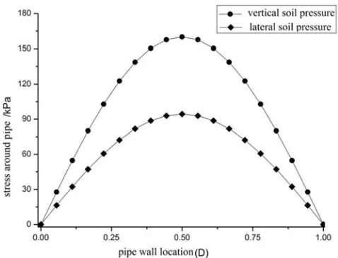
Figure 3. The simplified stress distribution around pipeline.
the side of the pipe calculated by Rankine model presents linearly increasing oblique rectilinear graph. This shows that compared with the actual results, there is a big error in soil pressure calculated by the Marston model.
The above calculations also show that the soil pressure acting on the buried pipeline is in addition to the normal stress, and there is considerable numerical shear stress around the pipe. However, the effect of circumferential shear stress is not considered in the present calculation method. It is obvious that this part of force should be considered when calculating the interaction between pipe and soil.
5. Conclusion
Based on the method of stress function, the calculation model of the soil pressure around the pipe is derived, and the analytic relationship between the cross sectional stiffness and the circumferential stress of the pipe is established. The circumferential stress varies according to the law of sine or cosine, and the circumferential stress obtained by elastic solution is very close to that calculated by finite element method. The simplified soil pressure of the pipe is parabola distributed in an outward convex direction, and the shear stress at the pipe circumference should be taken into account in the calculation of the interaction between the pipe and soil.
Acknowledgements
This work is financially supported by National Natural
Science Foundation of China (NSFC, 51408057) & Youth Talent Project of Yangtze University (2015 cqr 06).
References
[1] Liu Quanlin, Geotechnical Mechanics, Vol. 28, 2007, pp. 83-87.
[2] Jin Liu, Li Hongjing, Yao Baohua, Journal of Nanjing University of Technology (Natural Science Edition), Vol. 31, 2009, pp. 37-41.
[3] Huang Chongwei, Highway Engineering, Vol. 36, 2011, pp. 164-168.
[4] Wang Zhimin, Zhang Tuqiao, Wu Xiaogang, Water Conservancy and Hydropower Technology, Vol. 37, 2006, pp. 48-51.
[5] Yang Hui, Wang Ting, Lei Zhengqiang. Oil Field Equipment, Vol. 44, 2015, pp. 44-47.
[6] Wang Guangqin Ding Guabao Yang Jie. Elastic Mechanics [M]. Beijing: Tsinghua University Press, 2015.
[7] Xu Zhilun. Elastic Mechanics (Fifth edition) [M]. Beijing: Higher Education Press, 2016.
[8] Wang Zhechao. Elastic Mechanics [M]. Beijing: China Building Industry Press, 2016.
[9] She Yanhua. Doctoral Dissertation [D]. 2012, pp. 67-68. [10] Huang Qingyou, China Civil Engineering Journal, Vol. 15,