Analytical Solution to Find the Interference
Boundaries of Planar Cable-Driven Mechanisms
Omid Heidari PhD student
Department of Mechanical Engineering Idaho State University
Pocatello, ID 83209 Email: [email protected]
Saeed Behzadipour Associate professor
Mechanical Engineering Department Sharif University of Technology
Azadi St., Tehran, Iran Email: [email protected]
ABSTRACT
Cable interference in cable-driven mechanisms (CDM) is a major challenge in their applications. The wrench closure workspace (WCW) in a fully constrained mechanism may not be realized unless cable interference is con-sidered. This paper classifies all possible types of cable interferences for planar cable-driven mechanisms and presents an analytical solution to find the boundaries of the constant-orientation interference region. It is shown that interference between cables starts and ends when one end of a cable coincides with another cable which can be thought as lying a point on a line segment. This geometrical view is developed and applied to provide a frame-work for the analysis of cable interference. By subtracting the interference space form WCW, the interference-free workspace is obtained in which the robot is able to operate.
Keywords: planar cable-driven mechanisms; interference; wrench closure workspace
Nomenclature
Q Transformation matrix from the moving frame to the fixed one. ai The position vector ofAiexpressed in the moving frame.
bi The position vector of pointBiexpressed in the fixed frame.
f The position vector of Frame{O0}relative to the fixed frame. r+i The position vector of pointR+i expressed in the moving frame. r−i The position vector of pointR−i expressed in the moving frame. u A column vector showing the first row of the transformationQ. v A column vector showing the second row of the transformationQ.
1 Introduction
Cable-driven mechanisms (CDM) are manipulators in which the end-effector (EE) is connected to the base by cables with variable lengths. Their advantages over the conventional parallel manipulators include higher speed and acceleration (due to their light weight), lower costs, larger workspace, and easiness of reconfiguration. NIST ROBOCRANE [1], Mc-Donnell Douglas Charlotte [2], FALCON [3] and DeltaBot [4] are some examples of this type of robotic systems. Due to the unilateral force characteristic of cables, the theoretical foundation of such manipulators have formed around maintaining tensile force in all cables in order to provide structural rigidity. To maintain tensile forces in the cables of a CDM under any
desired loading, the number of cables must be at least one more than the degrees of freedom (DOF) [5]. The set of all poses in which a range of external wrenches can be generated using a limited range of cable tensions is called wrench feasible workspace (WFW) [6–9]. A special case of WFW happens when both cable tension and the wrench sets are unbounded which is called wrench closure workspace (WCW) [8, 9].The former depends on external loading, static or dynamic equilib-rium and cable properties while the latter only depends on the manipulator kinematics. Knowing the WCW is a necessary but not sufficient condition for safe operation of a CDM since interference may occur between two cables or between a cable and the EE referred to as Cable-Cable (C-C) and Endeffector-Cable (E-C) interference, respectively. Williams II and Gallina presented a method to analyze the interference of planar cable robots [10]. They considered the alignment of a cable with edges of the EE as a criterion to find E-C interference. Although it is theoretically able to find the E-C interference, the mathematical presentation is complex and hard to solve analytically. They did not include the C-C interference problem and the case of 3D as they assume all cables and the EE are in different parallel planes. To overcome the collision problem in 3D space, Merlete al. [11] formulated the minimum distance between two cables or between a cable and an edge of the EE using a numerical approach. Ghasemi et al. [12] investigated the C-C interference using the parametric equations of lines. When the line parameter is between zero and one, the C-C interference occurs. Also the E-C interference in 3D occurs when the direction of a cable aligns with one of the neighboring faces of the EE. This can be considered as an extension of Williams II and Gallina’s work. This condition, however, seems to be sufficient but not necessary for interference in 3D. As a result, the method becomes conservative in determining the interference-free workspace. The necessity and sufficiency proofs are reported by Yu Su et al. [13] for a polyhedral EE. All above-mentioned methods require numerical solutions. Thus, ana-lytical comprehensive solutions are still sought after in determining the borders of the interference space in CDMs. This paper presents an analytical approach to determine the interference space in planar CDMs with constant orientation. In [14], Perreault et al. addressed the problem geometrically and got similar solution however we focus more on the 2-D space and suggest a clear classification for interference problem. Section 2 presents the modeling concept of cable interference as well the classification of CDM’s and possible intereferences. The concept is developed in Section 3 and the formulation of the boundaries of interference regions are given in Section 4. A typical example of a planar CDM is then presented in Section 5 for detailed analysis of its interference regiosns. Section 6 presents a comparison between the interference regions and the WCW of the example followed by the conclusion.
2 Modeling Interference in planar CDM
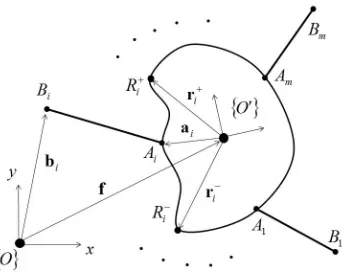
A planar single body CDM is composed of an end-effector, constrained to move on a plane, driven through pulling several cables. Thus the position of the EE is determined byx,yandθ. Fig. 3 depicts a schematic of a planar single body CDM. Each cable is attached to a point on the outline of the EE shown byAiand wound at the base around an actuated reel located atBi. aiis the position vector ofAiwith respect to the moving frame at{O0}andbiis the position vector of point
Biwith respect to the fixed frame at{O}. Each cable is assumed to be attached to the EE and the base by unique points, i.e. the cables do not share their end points. These points can be considered as revolute joints whose axes are orthogonal to the plane.
Fig. 1: Schematic of a single body CDM.
According to Fig. 3, R−i shows the point on the EE outline which would be the first point to touch cableiif the EE rotates clockwise aboutAi. Similarly,R+i shows the other point on the EE outline if the EE rotates counter-clockwise about
arguments applies toR+i andAi+1similarly. These two points are also presented by position vectorsr+i andr−i relative to the moving frame, respectively. If the EE outline betweenAiandR+i is a straight line, then any point in between can act asR
+
i as they touch the cable all at the same time. We consider the end point on this line asR+i . The position of frame{O0}relative to the fixed frame isf=
x,yT
and the orientation of EE is defined by angleθresulting in the following transformation matrix from the moving frame to the fixed one:
Q=
cosθ −sinθ sinθ cosθ
= uT vT (1)
in whichuandvare vectors showing the rows of the transformation matrix. Thus, pointsAi,R+i , andR −
i can be expressed in the fixed frame as:
OA
i=f+Q ai,ORi+=f+Q r+i ,OR −
i =f+Q r
−
i (2)
The main types of interference in CDM may be categorized as:
1. Interference between two cables or Cable-Cable (C-C) interference.
2. Interference between the end-effector and a cable or E-C interference which occurs when one cable comes in contact with the end-effector.
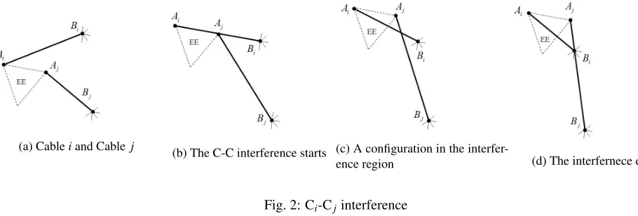
One may consider other types of interferences as well. For instance, Base-End effector interference or interference between the robot and an external obstacle. However, since such types of interference are not specific to CDMs and may happen in any type of robotic manipulators, they are excluded from this study. Also it should be noted that interference between the base and cables is not a different type from the abovementioned cases. Note that any collision between any cable and the cable collecting winches can be considered either as a C-C interference (if the geometry of the winch is ignored and the winch is modeled as the end point of a cable) or an interference between a cable and an external obstacle which is not of interest in this study. Among the two possible interferences, C-C interference has a slightly different nature in 2D CDMs compared to the 3D ones. In a spatial CDM, C-C interference may happen by collision between two cables at any point along the cables. This, however, may only happen at one of the two cable ends in a 2D CDM. As a result, in order to detect a C-C interference in 2D, it is sufficient to look for collision between a cable end point (on the EE or the base) with another cable. In other words, C-C interference starts and ends with a point-cable interference. One may also notice that the E-C interference in a planar CDM starts when a point of the end-effector’s outline, let’s sayR+i orR−i , hits cablei(Ci). As a result, in both types of interference, the boundary of interference is determined by point-cable collision. As an example, consider an interference between cables Ciand Cjin a CDM with a constant orientation of the end-effector as shown in, Fig. 2. In a series of pictures, it depicts how Cjstarts interfering Ci. WhenAjlies on Ci, the interference starts forming and ends whenBilies on Cj. It is clear that in C-C and E-C interferences a region of the workspace is determined in which at least one type of interference occurs (e.g. Fig. 2c and 2d). Such regions are calledinterference regionsin this work. It is also seen that the boundaries of interference regions are lines which will be determined later.
(a) Cableiand Cable j
(b) The C-C interference starts (c) A configuration in the
interfer-ence region (d) The interfernece ends
Fig. 2: Ci-Cjinterference
the CDMs can be designed such that the possibility of interferences and their complexities are reduced significantly. To elaborate, remember that in a planar CDM, the EE and cables do not need to lie on the same plane. The base can be assumed to be on a different parallel plane attached by perpendicular rods toBi’s so that the cable bases can be considered as points on the EE plane. Let us classify CDM’s according to the planes on which the cables and the EE lie:
• Class I - All on a single plane: Class I refers to a planar CDM in which all cables, the base, and the EE are on the same plane. In this class, both interferences, C-C and E-C, are possible. However, it is clear that the beginning and ending of any C-C interference corresponds to an E-C interference. As a result, it suffices to investigate E-C interferences to fully determine the interference region in this class.
• Class II Cables and the EE on different planes: If all cables are on one plane parallel to the plane of the EE, a class II mechanism is obtained. In this case, cables are attached to the EE using, for instance, rigid rods normal to the EE. It is clear the in this mechanism, C-C is the only possible interference.
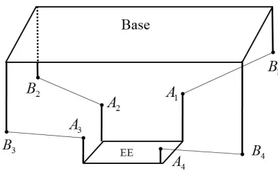
• Class III Cables on different planes. As depicted in Fig.3, in a Class III robot, each cable moves on a different yet parallel planes with the EE. The end-effector in such a mechanism needs a kinematic joint to keep it on the plane since the moment of the cable forces may give it an out of plane rotation. This configuration avoids all interferences except some of those between the cables and the connecting rods which is modeled as a point. Note that since this point is an isolated one, the corresponding interference region is only a line. This reduces the overall area of interference region significantly
Fig. 3: Class III of a CDM in which each cable is on a separate plane parallel with the end-effector.
As mentioned earlier, the boundaries of all interference regions are determined by a cable-point collision which will be formulated in the next section.
3 Detection of point-cable (P-C) collision
As it was stated in the previous sections, regardless of the type of interference (C-C or E-C interference), the region starts forming or ends when a point such asR+i ,R−i ,Ai, orBilies on a line segment. This concept makes the formulation of the problem clear and straightforward. Thus, P-C interference becomes the critical issue in the subject. Moreover, it is possible to narrow the interference space down into its boundary if P-C is the only type of interference which may occur. Let’s consider point Pand a line segment representing a cable with the fixed end (base) at B and the moving end atA, respectively. When pointPlies on the line segmentAB, we have:
(Ax−Px)(By−Py)−(Ay−Py)(Bx−Px) =0 (3)
The next step is to find the inequalities which limit pointPbetweenBandA. It can be shown thatPis betweenAandBif and only if:
(Bx−Px)(Ax−Px)≤0 (4)
It is shown in Theorem 1 of the Appendix that instead of the last two inequalities, one can use the following one along with Eq. (3) to figure out ifPis on line segmentAB:
(Bx−Px)(Ax−Px) + (By−Py)(By−Py)≤0 (6)
4 Boundaries of Interference Regions in CDM’s
The root of any interference is the collision of a point and a cable (P-C) which was formulated in the last section. This P-C collision however might be the result of two cables colliding each other (C-C) or a cable and the EE (E-C). In this section, C-C and E-C interferences are analyzed using P-C collision. In Table 1, each interference is resolved into several pairs of P-C collisions. Each pair corresponds to a boundary of the interference region. It should be noted that from the cases in the second column of the table, all butBi-Cj, present a collision between a cable and a point on the EE outline. Therefore, we first presentAj-Ci interference as a general formulation to determine the corresponding boundaries of the interference region. In the next step,Bi-Cjinterference which corresponds to a collision between the base and a cable will be presented.
Table 1: Boundaries of Different Interference Regions.
Interference Boundaries of the interference region are determined by
Cj-Ci Aj-Ci, Bi-Cj
E-Ci R+i -Ci, R−i -Ci
4.1 Aj-CiBoundary
To this end,BandAfrom Eq. (3) are replaced byBiandAiandPis also replaced byAjfor j6=ito obtain:
(f+Q ai−f−Q aj)x(bi−f−Q aj)y−(f+Q ai−f−Q aj)y(bi−f−Q aj)x=0 (7)
ReplacingQfrom Eq. (1) in the foregoing equation, upon simplifications leads to:
(vTs)x−(uTs)y+biyuTs−bixvTs+ (vTs)(uTaj)−(vTaj)(uTs) =0 (8)
wheres=ai−aj. Using Theorem 2 from the Appendix, the following simplifications are applied to Eq. (8):
(vTs)
x−(uTs)y=fTD Q s, biyuTs−bixvTs=bTiDTQ s, (vTs)(uTaj)−(vTaj)(sTu) = (v×u)T(s×aj) =sTi DTajwhere
D=
0 1 −1 0
which results in:
fTD Q s+bTiDTQ s+sTi DTaj=0 (9)
It is noteworthy that the first term in Eq. (9) depends on both position and orientation, the second term depends only on the orientation and the third one is a constant. Then, it can be written as
g1x+g2y+g3=0 (10)
(6) to confine pointAj to stay between the two ends of the cable. For this purpose, similar to Eq. (7), one can derive the following inequality:
(bi−f−Q aj)x(Q ai−Q aj)x+ (bi−f−Q aj)y(Q ai−Q aj)y≤0 (11)
ReplacingQfrom Eq. (1) and after simplifications, we have:
−fTQ s+bT
i Q s−sTaj≤0 (12)
Similarly, the first term depends on the position and orientation, the second term depends only on the orientation and the third one is a constant. Therefore, it can be written as:
h1x+h2y+h3≤0 (13)
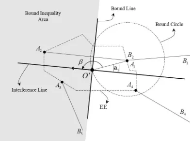
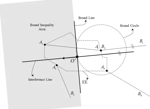
whereh1=−uTs,h2=−vTsandh3=bTiQ s−sTaj. For a given orientation, the above inequality shows the half of the plane separated by a line calledbound line. Considering the coefficients of theinterference lineandbound line, it turns out
Fig. 4: An example of a single body CDM with four cables.
that h1=g2 andh2=−g1meaning these two lines are perpendicular. To give a better view, a CDM with four cables is depicted in Fig. 4 which will be used as an example in the rest of this paper. For no change in EE orientation, j=1 and i=2, Fig. 5 depictsA1-C2interference line, bound line and bound inequality area. The part of interference line which is in the gray area shows the corresponding boundary of interference, i.e. A1is on Cable 2. As seen, the interference line is a
Fig. 5: Interference line, bound line and bound inequality area ofA1-C2
The intersection of the two lines is where the interference line is bounded. To find this intersection, one need to consider the coefficients in Eq. (9) and Eq. (12) as well as the fact thatDQ=QD, to obtain the following system of equations:
(fTQ−bTi Q+aTj)D s=0
(−fTQ+bT
i Q−aTj)s=0
(14)
Ifs=0, thenai=aj which means the attachment point of cableito EE coincides with that of cable jwhile we assumed that cables do not share their bases or ends soscannot be zero. As a result and using Theorem 3 (see Appendix), we have (fTQ−bTiQ+aTj) =0. Multiplying this equation byQT and a re-arranging the terms leads to:
bTiI−fTI=aTjQT (15)
which, after simplification, becomes:
(bix−x)2+ (biy−y)2=|aj|2 (16)
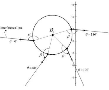
which is the equation of a circle centered atBi with a radius of|aj|. This circle is called bound circle as it represents the bounded end of the interference lines for various orientations of the end-effector. Figure 5 shows the bound circle and the interference line forθ=0 for the example of Fig. 4. When EE withθ=0 moves along the interference line from the intersection point,A1lies on cable 2 and interference starts. As a result, the interference line is unbounded from one end if there is no limit on the maximum length of Cable 2. Moreover, it can be shown that the angle between an interference line and the bound circle,βis constant and independent fromθ. As a simple proof, consider the radius of the bound circle drawn to the interference line (Fig. 5). The slope of this radius is m1=tanθ and the slope of the interference line is
m2=
(sxtanθ+sy)
(sx−sytanθ). Then one can derive the following relation between these two slopes:
sy
sx
= m2−m1
1−m1m2 (17)
On the other hand, m2−m1
1−m1m2 is equal to tanβresulting in tanβ= sy
sx . Thus,βis a constant value dependent on the EE outline. For instance,A1-C2interference lines forθ=0, 60, 120, and 180 are drawn in Fig 6. Since for eachθa different
Fig. 6: Different interference lines ofA1-C2corresponding to different orientations of the EE
dimension. Therefore, each interference line generates a helix with the following formula:
x=|aj|cosθ+bix
y=|aj|sinθ+biy
z=θ
(18)
As mentioned earlier, the above procedure can be identically used for any point on the EE outline such asR+i andR−i to investigate their collision with Ciand determine the corresponding boundary of the interference region. Therefore,R+i -Ci, andR−i - Cicollision can be computed in the same way.
4.2 Bi-CjBoundary
By replacingP,A, andBbyBi,Aj, andBj, respectively in Eq. (3), we have:
(f+Q aj−bi)x(bj−bi)y−(f+Q aj−bi)y(bj−bi)x=0 (19)
wheret=bi−bj. Then upon simplification, it results:
tTD f+tTD Q aj−tTD bi=0 (20)
Similar to the previous section, one can re-write this equation as a line:
l1x+l2y+l3=0 (21)
wherel1=−ty,l2=txandl3=tTD Q aj−tTD bi. For anyθ, the slope of this line is constant sincesxandsyare constant. In fact the slope of this line is the same as that of the line passing through pointsBiandBj. The next step is to find the bound inequality. ReplacingP,A, andBbyBi,Aj, andBj, respectively in Eq. (6), leads to:
−tTf−tTQ a
j+tTbi≤0 (22)
This inequality can also be rewritten as:
v1x+v2y+v3≤0 (23)
wherev1=−tx,v2=−ty, andv3=−tTQ a
j+tTbi. Similarly, for anyθ, the slope of this line is constant and is the same as that of the line passing through Bi andBj. Sincel1=v2 andl2=−v1, the bound line and the interference line are perpendicular. To find their intersection, the following system should be solved:
tTD(f+Q aj−bi) =0
tT(−f−Q aj+bi) =0
(24)
tcannot be zero otherwisebi=bj while we assumed that the attachment points of cableiand jon the base platform are distinct. As a result and according to Theorem 3,(f+Q aj−bi)should be zero which can be written as
y−biy=−vTaj
x−bix=−uTaj
(25)
These two equations can be combined and simplified as:
which yields the same bound circle as in the previous section whereAjcollided Ci. Figure 7 shows the bound line, interfer-ence line, and its parallelism with the line passing throughB1andB2for j=1 andi=2 in the example.
Fig. 7:B2-C1
5 Example: Interference Region of a Planar CDM
In this section, for a typical planar CDM which is a three DOFs mechanism with four cables, depicted in Fig. 4, the interference region are determined by its boundaries. All three classes of planar mechanisms (see Section 2) are investigated in order to elaborate on the effects of the cable arrangements on the interference region.
5.1 Class I:E-Cinterference
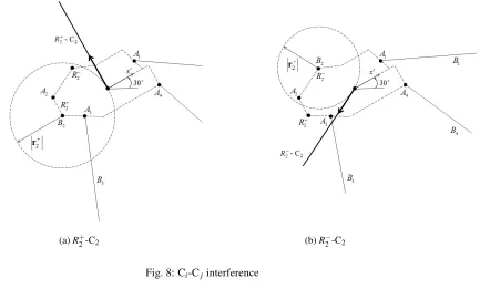
When all cables and the end-effector lie on the same plane, a class I mechanism is obtained. As previously stated, it is sufficient to determine the E-Ciboundaries (i=1, 2, , n) in this case. Such boundaries includesR+i -Ci,R−i -Ci; note that some ofR+i orR−i may coincide with someAj. To findR+i -CiandR−i -Ciboundaries, the procedure explained in section 4.1
was followed in whichAjwas replaced byR(+/ −)
i . Accordingly,ajwas replaced byr(+/ −)
i in Eq. (9). Letk+=ai−r+i and
k−=ai−r−i , then interference line equations forR
+
i -CiandR−i -Ciare:
fTD Q k+−bTiD Q k++aTjD k+=0
fTD Q k−−bTiD Q k−+aTjD k−=0 (27)
The bound inequality (12) was also found as:
−fTQ k++bTi Q k+−aTjk+≤0
−fTQ k−+bTi Q k−−aTjk−≤0 (28)
After simplification, the following bound circles are obtained:
(bix−x)2+ (biy−y)2=|r+i |2
(bix−x)2+ (biy−y)2=|r−i |2
(29)
(a)R+2-C2 (b)R−2-C2
Fig. 8: Ci-Cjinterference
Note that the bounded ends of these two interference lines would be the same if the interference of the EE outline (betweenR−2 andR+2) with the base of cable 2 was also considered. As said before, this type of collision (EE Base) was skipped in this paper as it is not specific to CDM’s.
Fig. 9: E-C2interference boundaries
Fig. 10: E-C interference-free workspace of the example CDM
5.2 Class II:C-Cinterference
In this class, the end-effector lies on a different parallel plane from the plane of cables in which C-C interference is the only possible one. Boundaries of the interference region are determined byAj-Ci, andBi-Cjinterference, which were investigated in sections 4.1 and 4.2 respectively. Figure 11 depictsAj-Ci andBi-Cj boundaries of the Cj-Ci interference region forθ=0 , j=1 andi=2. As shown earlier, the slope of theA1-C2interference line depends on the orientation of
Fig. 11: C1-C2interference.
(a)θ=0 (b)θ=60
Fig. 12: C-C interference
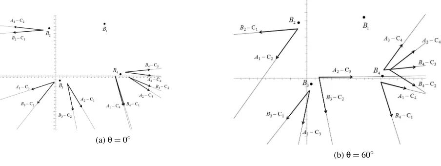
5.3 Class III: P-C interference
Now, if each cable lies on a distinct plane parallel to that of the end-effector, then the interference region is narrowed down into its boundaries since no C-C or E-C interference is possible. In such case, P-C collision provides the boundaries of the interference which cannot be crossed by the end-effector although the area of interference region is zero. As a result, the map of the possible interference shown in Fig. 12 changed to Fig. 13 when the mechanism changed to a Class III assuming that cables 1 is moving on the highest plane followed by cables 2, 3, 4, and the end-effector (similar to the scheme shown in Fig. 3). This arrangement of the cables avoided some of the interference altogether. For instance none ofA2-C1,A3-C1, A4-C1could happen anymore and the largest interference-free workspace was obtained
(a)θ=0◦
(b)θ=60◦
Fig. 13: P-C interference
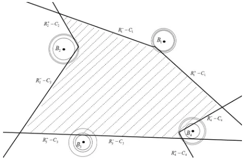
6 Wrench Closure Workspace and the Interference Region
(a)θ=0◦
(b)θ=60◦
Fig. 14: P-C interference, the hatched areas shows the WCW
I, when all cables and EE are on the same plane and the orientation isθ=30◦, the WCW is free of any collision as shown in Fig. 15. Similarly for Class II and III, there is no collision if the EE stays in the WCW.
(a) Class I (b) Class II
(c) Class III
However, when the orientation changes intoθ=180◦, as shown in Fig. 16, in Class I and Class II, the WCW has major overlaps with the interference regions. The only Class in which the mechanism can work without any interference in Class III. As it is shown in the figure, the boundaries of interference have made the WCW broken down into smaller pieces in which the EE can operate without collision however it cannot cross one region into another. These areas are hatched in different directions in the figure
(a) Class I (b) Class II
(c) Class III
Fig. 16: WCW vs. interference regions withθ=180◦
7 CONCLUSIONS
A detailed classification of the interference problem in CDMs was presented and the corresponding formulation was given. The formulation provides the boundaries of the interference region analytically and can be used to determine the region before operating the robot. It was shown that the interference regions for class I and II are sparse regions with linear boundaries while in class III the interference only happens along boundary lines. In other words, the interference region has zero area. Also, in an example it was shown that the interference region may or may not overlap with the wrench closure workspace.
References
[1] Albus, J., Bostelman, R., and Dagalakis, N., 1992. “The nist robocrane”.Journal of Robotics System,10(5).
[3] Kawamura, S., and Ito, K., 1993. “A new type of master robot for teleoperation using a radial wire drive system”. In Intelligent Robots and Systems’ 93, IROS’93. Proceedings of the 1993 IEEE/RSJ International Conference on, Vol. 1, IEEE, pp. 55–60.
[4] Dekker, R., Khajepour, A., and Behzadipour, S., 2006. “Design and testing of an ultra-high-speed cable robot”. International Journal of Robotics & Automation,21(1), p. 25.
[5] Rezazadeh, S., and Behzadipour, S., 2007. “Tensionability conditions of a multi-body system driven by cables”. In ASME 2007 International Mechanical Engineering Congress and Exposition, American Society of Mechanical Engi-neers, pp. 1369–1375.
[6] Bosscher, P., Riechel, A. T., and Ebert-Uphoff, I., 2006. “Wrench-feasible workspace generation for cable-driven robots”.IEEE Transactions on Robotics,22(5), pp. 890–902.
[7] Barette, G., and Gosselin, C., 2000. “Kinematic analysis and design of planar parallel mechanisms actuated with cables”. In Proceedings of ASME Design Engineering Technical Conference, pp. 391–399.
[8] Gouttefarde, M., and Gosselin, C. M., 2004. “On the properties and the determination of the wrench-closure workspace of planar parallel cable-driven mechanisms”. In ASME 2004 International Design Engineering Technical Conferences and Computers and Information in Engineering Conference, American Society of Mechanical Engineers, pp. 337–346. [9] Gouttefarde, M., and Gosselin, C. M., 2006. “Analysis of the wrench-closure workspace of planar parallel cable-driven
mechanisms”.IEEE Transactions on Robotics,22(3), pp. 434–445.
[10] Williams, R. L., and Gallina, P., 2002. “Planar cable-direct-driven robots: design for wrench exertion”. Journal of intelligent and robotic systems,35(2), pp. 203–219.
[11] Merlet, J.-P., 2004. “Analysis of the influence of wires interference on the workspace of wire robots”. InOn Advances in Robot Kinematics. Springer, pp. 211–218.
[12] Ghasemi, A., Farid, M., and Eghtesad, M., 2008. “Interference free workspace analysis of redundant 3d cable robots”. In 2008 World Automation Congress, pp. 1–6.
[13] Su, Y., Mi, J. W., and Qiu, Y. Y., 2011. “Interference determination for parallel cable-driven robots”. In Advanced Materials Research, Vol. 308, Trans Tech Publ, pp. 2013–2018.
[14] Perreault, S., Cardou, P., Gosselin, C., and Otis, M., 2010. “Geometric determination of the interference-free constant-orientation workspace of parallel cable-driven mechanisms”.
Appendix
Theorem 1: The solution to inequalityu4u1+u2u3≤0 is equal to those of system of inequalitiesu4u1≤0 &u2u3≤0, provided thatu1u2−u3u4=0.
Proof: consider the following system:
u4u1+u2u3≤0 (I)
u1u2−u3u4=0 (II)
Ifu1>0, then by multiplying (I) byu1, (II) byu3and replacing (u1u2u3)from latter into former, we have:
u4(u23+u21)≤0 (1)
Sinceu16=0, then(u2
3+u21)>0 which results inu4≤0 and consequentlyu1u4≤0. Foru1<0, the same result will be achieved. Ifu1=0, then from (I) we haveu3u2≤0. Similarly, using the same procedure foru3andu2, the result will be u3u2≤0.
Theorem 2:(a·c)(b·n)−(a·n)(b·c) = (a×b)·(c×n)
Proof: If vector triple product(a·c)b−(b·c)a= (a×b)×cis multiplied by arbitrary vectorn:
(a·c)b·n−(b·c)a·n=n·((a×b)×c)
Then, by scalar triple product rule, the term in right hand side can be written as
Theorem 3:
(aTb=0 → |a||b|cosα=0 → |a||b|cosα=0
aTD b=0 → |a||b|cos(α−π
2) =0 → |a||b|sin(α) =0