Benchmark Synthetic Training Data for Artificial

Benchmark Synthetic Training Data for Artificial

1

Intelligence-based Li-ion Diagnosis and Prognosis

2

Matthieu Dubarry 1,*, and David Beck 2

3

1 _{University of Hawaii, Hawaii Natural Energy Institute; [email protected]}

4

2 _{University of Hawaii, Hawaii Natural Energy Institute; [email protected]}

5

* Correspondence: [email protected]

6

7

Abstract: Accurate lithium battery diagnosis and prognosis is critical to increase penetration of

8

electric vehicles and grid-tied storage systems. They are both complex due to the intricate, nonlinear,

9

and path-dependent nature of battery degradation. Data-driven models are anticipated to play a

10

significant role in the behavioral prediction of dynamical systems such as batteries. However, they

11

are often limited by the amount of training data available. In this work, we generated the first big

12

data comprehensive synthetic datasets to train diagnosis and prognosis algorithms. The

13

proof-of-concept datasets are over three orders of magnitude larger than what is currently available

14

in the literature. With benchmark datasets, results from different studies could be easily equated,

15

and the performance of different algorithms can be compared, enhanced, and analyzed extensively.

16

This will expend critical capabilities of current AI algorithms, tools, and techniques to predict

17

scientific data.

18

Keywords: Machine Learning, Training Data, alawa, AI

19

20

21

In recent years, artificial intelligence (AI) has attracted a lot of attention for energy applications

22

[1-4]. For the diagnosis and prognosis of lithium-ion battery (LiB), one bottleneck is the training data

23

that is not populated enough and not representative of the projected sporadic usage [3,5]. This can

24

hinder performance as models can only be as good as the data they were trained with. Most studies

25

had training datasets below 20 samples. Among the studies with more, [5-12], the study by Severson

26

et al. [5,11] stands out with 124 different conditions tested, although only charging conditions were

27

varied. Even though online databases [5,13-18] are a step in the right direction, this is vastly

28

insufficient because LiB degradation is path-dependent and small changes in conditions were shown

29

to lead to drastic differences in durability [19]. This path dependence is an essential aspect to

30

consider for the validation of online diagnosis and prognosis tools [20,21]. With a limited set of

31

training data, the universality of the diagnosis and prognosis tool cannot be proven.

32

The need for high throughput computational data generation was highlighted in recent reviews

33

[1,2], although no effort towards computational cycling training data has been reported. In this

34

work, we will report the first synthetic benchmark training datasets that englobe the entire

35

degradation spectrum. This will be done using computer-assisted voltage curve generation to

36

remove the need for lengthy and costly experimental campaigns. The datasets will be computed

37

using the mechanistic modeling approach we pioneered, along with other groups, in the mid-2000s

38

[22-25]. The approach has been well validated [26-28] and has been intensively used in recent years

39

with the rise in popularity of the electrochemical voltage spectroscopies (EVS) [29,30]. The use of the

40

mechanistic approach will enable the creation of training datasets several orders of magnitude larger

41

than the current ones encompassing all possible degradation scenarios. This is especially important

42

for prognosis tools as battery capacity loss is known to accelerate at some point upon aging. This is

43

the essential feature than any good prognosis needs to capture. This acceleration usually originates

44

from degradations that have an “incubation” period that does not affect capacity [21]. A complete

45

training dataset should contain examples of paths with an acceleration induced by different

46

components of the degradation, whether it is the loss of lithium, losses in active materials, or

47

resistance.

48

49

50

Compared to traditional battery modeling [31,32], the mechanistic framework is a backward

51

modeling approach where the input is the degradation and the output the cell’s voltage and

52

capacity. This makes the method perfect for generating training data and more efficient than

53

electrochemical models because there is no need to find actual physical phenomena that could lead

54

to a given degradation. The initial set up is also simpler without a need for complex

55

parameterization and the only prerequisite being half-cell data versus a reference electrode for both

56

electrodes. In 2017, we proposed to use this approach to perform sensibility analyses by simulating a

57

wide range of hypothetical degradation scenarios [20]. This work is building on our previous effort

58

to enable the creation of comprehensive training data.

59

In this work, we will focus on diagnosis and prognosis, two applications that require different

60

sets of training data. To illustrate the difference between the two requirements, one can think of two

61

time-dependent processes, one linear and one exponential, intersecting. At the intersection, the

62

diagnostic will be the same, but the prognosis needs to be different. In addition, we will also address

63

another hurdle for AI algorithms, the quest for meaningful learnable parameters. Although some

64

studies seem to fit the full constant current voltage data [33], most studies favor the use of features of

65

interest (FOI) and only focus on a specific part of the electrochemical response. This could be

66

capacity and resistance evolution [10,34-37], curvature [38,39], sections of the voltage response

67

[8,40-42], electrochemical impedance spectroscopy [43,44], variance [5,11], or EVS [33,45-48]. The

68

latter has attracted a lot of attention in recent years since the early work on the technique [22,49,50].

69

Still, the correlation of the variations with degradation is not trivial and requires significant

70

sensibility analysis to derive universal parameters [20]. Some FOIs proposed in the literature were

71

proven not applicable outside of the tested data [21], which illustrates the need for more extensive

72

training sets and proper sensitivity analysis of the learnable parameters. With controlled and

73

complete training, the theoretical framework to establish relationships between data and models can

74

be explored in much more detail, and results from different studies could be easily equated.

75

The purpose of this publication is to introduce a big data methodology and showcase its

76

possibilities. The optimization of the technique to reduce computation time and its integration with

77

AI algorithms is out of the scope of this work.

78

Methodology

79

The mechanistic approach conceptually follows the one described by Christensen and Newman

80

to simulate cell degradation in the early 2000s [31,32]. Instead of computing-intensive

81

electrochemical models to simulate half-cell electrode behavior, the mechanistic approach [22-25]

82

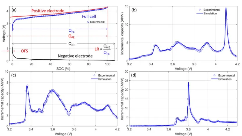
uses experimental half-cell data for each electrode. Figure 1(a) presents the mechanistic

83

representation of a cell. The matching consists of two parameters, the loading ratio LR between the

84

capacities of both electrodes and their offset OFS that is representative of the amount of lithium lost

85

during the solid electrolyte interphase formation. The circles in Figure 1(a) showcase how the

86

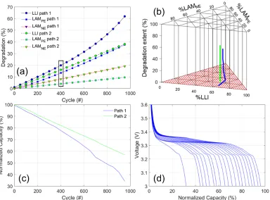
experimental data overlap the emulated cell perfectly. To enhance the differences, the same data can

87

be derived and plotted as incremental capacity, dQ/dV = f(V), Figure 1(b-d). For this EVS, each peak

88

represents a phase transformation in one of the electrodes. A perfect match between the emulated

89

and the experimental data proves that the emulated cell is perfectly replicating the experimental cell

90

voltage variations. Figure 1(b-d) presents examples of the quality of the obtainable fits for cells based

91

on different Li-ion chemistries from our previous work [51-53].

92

94

Figure 1: (a) Mechanistic model principles. The full cell response, in blue, corresponds to the

95

response of the positive electrode, in red, minus the one of the negative electrode, in black, after

96

matching. Fit for cells based on (b) a blended Graphite (Gr)-Silicon (Si) NE and Ni.8Mn.1Co.1O2

97

(NMC811) PE [53], (Gr) negative electrodes (NE) and (c) NixAlyCo1-x-yO2 (NCA) [51] as well as a (d)

98

blend of LiCoO2 (LCO) and NCA as (PE) [52].

99

100

While the active materials are considered stable with aging, their quantity, as well as the

101

amount of Lithium reacting, will change upon degradation. Degradation will then not affect the

102

electrode OCV curves, but it will impact their matching. If less active material is available, the

103

loading ratio between the electrodes will change. If some reactant is lost, the synchronicity of the

104

electrodes will change. These matching changes can be rendered in the mechanistic approach via

105

some scaling of the electrode curves and a translation of one electrode compared to the other, in

106

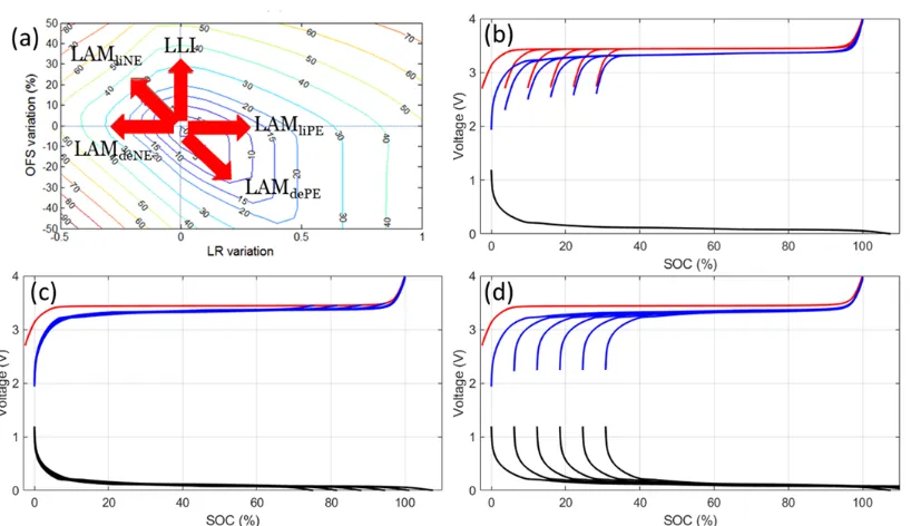
other words changing LR and OFS in Figure 1(a). Figure 2(a) presents the impact of the variation of

107

LR and OFS on cell capacity. In can be seen that there is an infinity of combination of LR and OFS

108

that can lead to any capacity loss; this is the path dependence of the degradation. This also explains

109

why measuring capacity will never be a good enough diagnosis of true degradation. Changes in the

110

amount of active material are referred to as loss of active material (LAM). LAM can occur at the PE

111

and NE. Change in the amount of lithium reacting is referred to as loss of lithium inventory (LLI).

112

The thermodynamic degradation of Li-ion batteries can be decomposed into these three main

113

degradation modes. LLI is inducing translation and the LAMs scaling, Figure 2(b-d). More details on

114

the technique and the associated equations can be found in [25].

115

117

Figure 2: (a) Impact of changes of LR and OFS on the capacity loss. Arrows represent the impact

118

of LLI and LAMs on LR and OFS. (b) Impact of LAMPE and (c) impact of LAMNE with the scaling of

119

the affected electrode compared to the other. (d) Impact of LLI with the translation of the NE

120

compared to the PE. In all cases, the full cell response, in blue, corresponds to the response of the

121

positive electrode, in red, minus the one of the negative electrode, in black, after matching.

122

123

The validity of the predicted impact of LAM and LLI on the electrochemical behavior of

124

experimental cells was verified by independent studies [26-28]. Most notably, Kassem et al. [26]

125

confirmed that LLI does induce electrode slippage between the NE and Schmidt et al. [54] verified

126

that LAM does influence the LR by assembling cells with different amounts of PE versus a constant

127

NE. Moreover, over the past decade, numerous studies [29,30] successfully used this approach to

128

diagnose the degradation of commercial cells. Figure 3(a,b) presents two examples of the fit of the

129

voltage response of aged commercial cells from previous works [53,55]. Figure 3(c,d) presents the

130

comparison of an experimental (from [53]) and a synthetic dataset constructed solely from half-cell

131

data and simple equations that modified the matching of the electrodes based on the quantification

132

of LLI and the LAMs. This highlights how the mechanistic approach is efficient to replicate the

133

voltage variations associated with cell degradation.

134

136

Figure 3: Example of voltage emulation after aging for (a) a Gr//NCA discharge [55] after 1,500

137

equivalent full cycles based on electric vehicle driving and frequency regulation. (b) A

138

Gr//LCO+NCA charges [53] after 1000 full cycles at 1.5C. (c) Experimental [53] and (d) synthetic

139

voltage variations upon aging calculated from simple linear equations extracted from the diagnosis.

140

141

From the mechanistic approach point of view, each thermodynamic degradation can be

142

described by a unique combination of the LLI, LAMPE, and LAMNE triplet. Conversely, scanning

143

every possible combination of the triplet yield any potential degradation from which the voltage

144

response can be reconstructed. This is the unique feature that is used in this work to build synthetic

145

training datasets.

146

For datasets aimed at diagnosis, the approach used in previous work on an automated

147

diagnosis tool for BMS [20] can be expanded. The [LLI, LAMPE, LAMNE] triplets can be normalized so

148

that their sum is equal to one and they can then be represented in a ternary diagram, Figure 4. By

149

scanning every point of this diagram (red dots) between 0 to 100% degradation for each mode

150

(vertical lines), each possible degradation can be represented, and the associated voltage response

151

calculated to be used in a training dataset. E.g., for the [0.5,0.2.,0.3] triplet, LLI would be varied from

152

0 to 100% with 1% increments, LAMPE from 0 to 40% with 0.4% increments, and LAMNE from 0 to

153

155

Figure 4: (a) Mechanistic model principles to emulate every possible degradation. Only partial

156

degradation calculations were represented for illustration purposes.

157

158

For datasets aimed at prognosis, the evolution of each degradation mode needs to be calculated

159

independently as the ratio between the normalized values of the triplet might not be constant. The

160

triplet values could be calculated, per example, for different linear degradation paces, with paces

161

linear combined with exponential variations, or with a delayed exponential increase, more

162

representative of the real degradation of commercial cells [19,56,57]. Since the voltages associated

163

with all the triplet values were already calculated for diagnosis, no additional simulations are

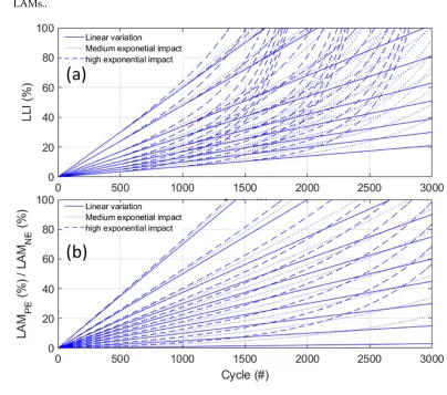
164

actually necessary and the different degradation paths are all inscribed in Figure 4. They can be

165

reconstructed by following the evolution of the triplet values in the ternary design space and the

166

corresponding voltage variations can be accessed. Figure 5 presents an example of the process for

167

two degradation paths for a Gr//LiFePO4 (LFP) cell. Figure 5(a) plots the evolution of the triplets for

168

each path. For each cycle, as exemplified by the black box in Figure 5(a), a triplet value can be

169

determined and the quantification can be used to find the corresponding point in the ternary design

170

space, Figure 5(b). In this example, path 2 (green) was simulated with linear variations for the three

171

components of the triplet, its path is, therefore, vertical as the ratio between the degradation modes

172

is constant. Path 1 (blue) had some exponential component for LLI and LAMPE and, therefore, the

173

path is more complicated. Nonetheless, based on the triplets and the diagnosis dataset, the capacity

174

loss, Figure 5(c), and the voltage variations, Figure 5(d), can be deciphered. This approach for

175

calculating a prognosis dataset will be faster than simulating each degradation path one by one as it

176

178

Figure 5: Example of the prognosis dataset calculation for two different paths for a Gr//LFP cell

179

with (a) the triplet variations, (b) their path in the ternary design space, (c) the reconstructed capacity

180

loss, and (d) the voltage variations for path 1.

181

182

It must be noted that the description above was simplified for narrative purposes and was

183

centered on the thermodynamic degradation observable at low currents and constant temperature

184

for ease of representation. The full mechanistic approach is much more complex [25]. To be able to

185

simulate different levels of usage, an equivalent circuit model (ECM) is included to handle different

186

rates for each electrode [22-26]. For electrode blends, or changes in electroactive phases upon aging,

187

each component of the electrode must be considered separately (i.e., LAMPE will be splat in LAMLCO

188

and LAMNCA for an LCO-NCA blended electrode). Moreover, for datasets at higher currents or

189

different temperatures, some kinetic parameters such as the ohmic and faradic resistance increase

190

must also be scanned as they will influence the voltage response of the cells. Finally, in some cases,

191

lithium plating, both thermodynamic and kinetic, must be taken into consideration [25]. The validity

192

of the mechanistic approach in all of those cases has been proven in the literature [19,58,59]. As

193

explained in [25,58], resistance changes can be accommodated by shifting the voltage curves up or

194

down depending on the electrode and the regime. Kinetic limitations can be handled by modifying

195

the simulated rate while counterbalancing the polarization changes. Simulating higher rates allows

196

emulating slower kinetics. Simulating lower rates allows emulating faster kinetics. This allows to

197

model different rates and temperatures [58]. Figure 6(a) presents an example from [58] where

198

different temperatures were simulated from 25°C data at different rates. For lithium plating, the

199

solution is to simulate the NE as a blend between Gr and metallic lithium with the metallic lithium

200

initially outside of the potential window, Figure 6(b). If LAMGraphite becomes prominent, or if its

201

resistance pushes its potential below 0V, the metallic lithium will then be dragged into the potential

202

window and start interacting with the PE [19,21,25]. As discussed in the literature [5,19,25,57],

203

thermodynamic lithium plating begins when there is enough LAMNE so that the NE is fully lithiated

204

before the PE is delithiated. The amount of LAMNE necessary for that to happen depends on the

205

initial cell configuration (LRini and OFSini) and also on the evolution of LLI and LAMPE [60]. Figure

206

degradation path. Lithium plating will start when LAMNE becomes larger than PT. This does not by

208

itself induce any capacity loss as metallic lithium can be reduced and oxidized. This lithium,

209

however, is usually quickly passivating, which results in additional LLI. To take this effect into

210

account, a correction for LLI can be introduced and the additional LLI is defined as the difference

211

between LAMNE and the PT, when positive, multiplied by a reversibility factor. Figure 6(c)

212

showcases an example of the acceleration in LLI based on different reversibilities. Figure 6(d)

213

presents the associated capacity loss showcasing the acceleration.

214

215

216

Figure 6: (a) Emulation of the impact of temperature at C/5 for a Gr//NCA cell from [58], and (b)

217

Electrode matching with a blended Gr-Li electrode with the Li outside of the potential window as a

218

reserve. Evolution of (c) LLI and LAMNE depending on the reversibility of lithium plating (0%, 50%

219

or 100%) and (d) the associated capacity loss.

220

Proof-of-concept datasets

221

For this proof-of-concept work, a Gr//LFP cell similar to the one used in [20] was chosen

222

because the sensibility analysis of different FOI was already reported and some non-ML diagnosis

223

tools were validated. The data could also be compared to the one from Severson et al. [5].

224

The diagnosis dataset contains more than 500,000 voltage vs. capacity curves. It can be used to

225

train machine learning algorithms, but more importantly, it can also be used to perform sensibility

226

analysis [20] to find out which FOIs are representative of different degradations or if they can be

227

used as universal proxies for capacity loss. An example is presented in Supplementary note 1.

228

The prognosis dataset contains more than 130,000 different degradation paths with upwards of

229

3,000,000 individual voltage vs. capacity curves. It can be used to test the validity of varying FOIs

230

proposed in the literature for early prognosis. An example is presented in Supplementary note 2.

231

Both datasets are available to download (see Data availability section for access information).

232

Limitations and outlook

233

In this work, we presented a proof-of-concept methodology to generate big data training

234

datasets for intercalation batteries. The mechanistic approach combines both modeling and

235

experimental techniques to provide a universal tool for the creation of synthetic voltage curves

236

practically indistinguishable from real data. This approach offers the benefits of the broad

237

applicability of the model to various cell chemistries, designs, and operating modes, as well as the

238

could be applied to the generation of training datasets encompassing the entire degradation

240

spectrum as well as different operating conditions such as rate and temperature. Scenarios leading to

241

lithium plating with adjustable reversibility can be added and the addition of random noise on the

242

data could be considered to make the datasets even more realistic and consider the impact of real-life

243

testing machines' precision and accuracy.

244

As a proof-of-concept, we generated a diagnosis dataset containing more than individual

245

500,000 voltage vs. capacity curves and a prognosis dataset with more than 130,000 individual

246

degradation paths for a commercial graphite//LFP battery. These datasets are more than three orders

247

of magnitude larger than the one currently available in the literature and they could be extended at

248

will. We showcased the use of the proposed datasets for FOI sensibility analysis and a diagnosis

249

technique based on the joint evolution of three FOIs since variations of single FOI were proven

250

inefficient. We also used them to propose an early prognosis method based on the extrapolation of

251

the diagnosis of the degradation modes.

252

Although there is still a lot of work to be done to optimize the technique, results are extremely

253

promising and should accelerate the development of accurate algorithms. The proof-of-concept

254

dataset used in this work were limited to thermodynamic degradations at constant temperature for

255

single-phase electrodes. Taking everything into account (LAMs, LLI, polarization, kinetics, phases,

256

temperatures…) for all the possible evolutions (linear, exponential, delays…) will take enormous

257

calculation time and generate overwhelming datasets. Some optimization and intelligence could be

258

applied to limit the number of degradation paths to test. A solution could be large designs of

259

experiments first to screen the impact of the different parameters then to focus on their

260

representativity in the paths to simulate. Here we provide an open framework to the community to

261

apply advanced optimization techniques to reduce the calculation burden.

262

Finally, we would like to point out that our intent is no way to remove the need for

263

experimental testing all-together. On the contrary, experimental testing is still essential, and the only

264

way, to decipher which conditions cater to specific degradation paths and its input is, therefore,

265

fundamental to decipher the applicability of batteries for a given application. Our methodology can

266

be used alongside to develop the needed algorithms once a cell was selected.

267

268

Methods

269

Half-cell data. Data from four different types of commercial cells were used in this work. The

270

Gr//NCA cell was a Panasonic 3350 mAh NCR 18650B [51,58,60-62]. The Si-Gr//NMC811 was a

271

Samsung-SDI 3350 mAh INR18650-35E [52], the Gr//LCO+NCA was an LG-Chem 2800 mAh

272

ICR18650 C2” [53], and the Gr//LFP was an A123 2300 mAh ANR26650M [19,63]. All were

273

extensively studied in previous work. Interested readers are referred to the original publications for

274

more details. The cells were slowly discharged to 0% SOC before being carefully disassembled in an

275

Argon-filled glove box where the electrodes, separator, and casing will be separated [64]. Electrode

276

discs (18 mm in diameter) were punched from the harvested electrodes and rinsed in a dimethyl

277

carbonate (DMC) solution. The backside of two-sided electrodes was then wiped clean using cotton

278

swabs soaked in nN-methyl-2-pyrrolidone (NMP) solvent before being the electrode was rinsed

279

again in a fresh DMC solution. The electrodes were tested using a lithium counter electrode. Metallic

280

lithium was applied onto a stainless-steel disk. An electrolyte solution of 1.0 M LiPF6 in ethylene

281

carbonate (EC) + DMC (1:1 by weight) + 2% wt. vinylene carbonate (VC) was used to soak the

282

separator, which consisted of one layer of Whatman GF-D fiberglass discs (12.7 mm in diameter,

283

Whatman), Kent, United Kingdom). Once sealed, the half-cells were taken out of the glove box and

284

connected to a multi-channel Bio-Logic VMP3 potentiostat (Bio-Logic, Claix, France) for testing at

285

different rates from low to high. The complete testing protocol can be found in [64].

286

287

Simulations. All simulations were performed under a MATLAB© environment using the ‘alawa

288

toolbox [65]. As in [20], the LFP and graphite electrodes were matched with an LR of 0.95, OFS of

289

The diagnosis training dataset was compiled with a resolution of 0.01 for the triplets and C/25

291

charges. This accounts for more than 5,000 different paths at the base of the triangle in Figure 4. Each

292

path was simulated with 0.85% increases for each degradation up to 85%. This accounts for 100

293

simulations per path. The training dataset, therefore, contains more than 500,000 voltage vs. capacity

294

curves and took around 12h to compute on a standard laptop. The 500MB dataset is available to

295

download (see Data availability section for access information).

296

The prognosis dataset was harder to define as there are no limits on how the three degradation

297

modes can evolve. For this proof of concept work, we considered eight parameters to scan. For each

298

degradation mode, degradation was chosen to follow equation (1).

299

300

% = × + ( × _{− 1) (1)}

301

302

Considering the three degradation modes, this accounts for six parameters to scan. In addition,

303

two other parameters were added, a delay for the exponential factor for LLI, and a parameter for the

304

reversibility of lithium plating. The delay was introduced to reflect degradation paths where plating

305

cannot be explained by an increase of LAMs or resistance [55]. The chosen parameters and their

306

values are summarized in Table S1. Figure S1(a,b) presents the evolution of parameters p1 to p7. At

307

the worst, the cells endured 100% of one of the degradation modes in around 1,500 cycles. Minimal

308

LLI was chosen to be 20% after 3,000 cycles. This is to guarantee at least 20% capacity loss for all the

309

simulations. For the LAMs, conditions were less restrictive, and, after 3,000 cycles, the lowest

310

degradation is of 3%. The reversibility factor p8 was calculated with equation (2) when LAMNE > PT.

311

312

%

(

−

)

(2)

313

314

Where PT was calculated with equation (3) from [60].

315

316

= 100 − 100−%

100× −% ×

(

)

(3)

317

318

Varying all those parameters accounted for more than 130,000 individual duty cycles. With one

319

voltage curve for every 100 cycles, it took around 12h to compute on a standard laptop to simulate

320

the more than 3,000,000 voltage vs. capacity curves. The 3GB dataset is available to download (see

321

Data availability section for access information).

322

323

Data availability. The datasets used in this study are available at

324

http://dx.doi.org/10.17632/bs2j56pn7y.1 and http://dx.doi.org/10.17632/6s6ph9n8zg.1 for the

325

diagnosis and prognosis dataset, respectively.

326

Author Contributions: Conceptualization, M.D.; methodology, M.D.; software, M.D.; validation, M.D. and

327

D.B.; formal analysis, M.D. and D.B.; resources, M.D.; data curation, M.D.; writing—original draft

328

preparation, M.D.; writing—review and editing, M.D. and D.B.; visualization, M.D.; supervision, M.D.;

329

project administration, M.D.; funding acquisition, M.D.

330

Funding: This work was funded by ONR Asia Pacific Research Initiative for Sustainable Energy Systems

331

(APRISES), award number N00014-18-1-2127. M.D. is also supported by the State of Hawaii.

332

Acknowledgments: M.D. is thankful to all the past staff that helped define and affine the concepts used in this

333

work, most notably Bor Yann Liaw, Cyril Truchot, Arnaud Devie, George Baure, and David Anseán.

334

Conflicts of Interest: The authors declare no conflict of interest.

335

References

336

1. Chen, C.; Zuo, Y.; Ye, W.; Li, X.; Deng, Z.; Ong, S.P. A Critical Review of Machine Learning of Energy

337

2. Ng, M.-F.; Zhao, J.; Yan, Q.; Conduit, G.J.; Seh, Z.W. Predicting the state of charge and health of

339

batteries using data-driven machine learning. Nature Machine Intelligence 2020,

340

10.1038/s42256-020-0156-7, doi:10.1038/s42256-020-0156-7.

341

3. Vidal, C.; Malysz, P.; Kollmeyer, P.; Emadi, A. Machine Learning Applied to Electrified Vehicle Battery

342

State of Charge and State of Health Estimation: State-of-the-Art. IEEE Access 2020, 8, 52796-52814,

343

doi:10.1109/access.2020.2980961.

344

4. How, D.N.T.; Hannan, M.A.; Hossain Lipu, M.S.; Ker, P.J. State of Charge Estimation for Lithium-Ion

345

Batteries Using Model-Based and Data-Driven Methods: A Review. IEEE Access 2019, 7, 136116-136136,

346

doi:10.1109/access.2019.2942213.

347

5. Severson, K.A.; Attia, P.M.; Jin, N.; Perkins, N.; Jiang, B.; Yang, Z.; Chen, M.H.; Aykol, M.; Herring,

348

P.K.; Fraggedakis, D., et al. Data-driven prediction of battery cycle life before capacity degradation.

349

Nature Energy 2019, 4, 383-391, doi:10.1038/s41560-019-0356-8.

350

6. Klass, V.; Behm, M.; Lindbergh, G. A support vector machine-based state-of-health estimation method

351

for lithium-ion batteries under electric vehicle operation. J. Power Sources 2014, 270, 262-272,

352

doi:10.1016/j.jpowsour.2014.07.116.

353

7. Klass, V.; Behm, M.; Lindbergh, G. Evaluating Real-Life Performance of Lithium-Ion Battery Packs in

354

Electric Vehicles. J. Electrochem. Soc. 2012, 159, A1856-A1860, doi:10.1149/2.047211jes.

355

8. Hu, C.; Jain, G.; Schmidt, C.; Strief, C.; Sullivan, M. Online estimation of lithium-ion battery capacity

356

using sparse Bayesian learning. J. Power Sources 2015, 289, 105-113, doi:10.1016/j.jpowsour.2015.04.166.

357

9. Richardson, R.R.; Birkl, C.R.; Osborne, M.A.; Howey, D.A. Gaussian Process Regression for In-situ

358

Capacity Estimation of Lithium-ion Batteries.

359

10. Pan, H.; Lü, Z.; Wang, H.; Wei, H.; Chen, L. Novel battery state-of-health online estimation method

360

using multiple health indicators and an extreme learning machine. Energy 2018, 160, 466-477,

361

doi:10.1016/j.energy.2018.06.220.

362

11. Attia, P.M.; Grover, A.; Jin, N.; Severson, K.A.; Markov, T.M.; Liao, Y.H.; Chen, M.H.; Cheong, B.;

363

Perkins, N.; Yang, Z., et al. Closed-loop optimization of fast-charging protocols for batteries with

364

machine learning. Nature 2020, 578, 397-402, doi:10.1038/s41586-020-1994-5.

365

12. Cripps, E.; Pecht, M. A Bayesian nonlinear random effects model for identification of defective

366

batteries from lot samples. J. Power Sources 2017, 342, 342-350, doi:10.1016/j.jpowsour.2016.12.067.

367

13. Kollmeyer, P.; Vidal, C.; Naguib, M.; Skells, M. LG 18650HG2 Li-ion Battery Data and Example Deep

368

Neural Network xEV SOC Estimator Script. Available online:

369

https://data.mendeley.com/datasets/cp3473x7xv/3 (accessed on 04/12).

370

14. Kollmeyer, P. Panasonic 18650PF Li-ion Battery Data”, Mendeley Data, v1. Available online:

371

https://data.mendeley.com/datasets/wykht8y7tg/1#folder96f196a8-a04d-4e6a-827d-0dc4d61ca97b

372

(accessed on 04/12).

373

15. Saha, B.; Goebel, K. Battery Data Set. NASA Ames Prognostics Data Repository. NASA Ames Research

374

Center. Moffett Field, CA, USA. Availabe online:

375

https://ti.arc.nasa.gov/tech/dash/groups/pcoe/prognostic-data-repository/ (accessed on 04/12).

376

16. Barkholtz, H.M.; Fresquez, A.; Chalamala, B.R.; Ferreira, S.R. A Database for Comparative

377

Electrochemical Performance of Commercial 18650-Format Lithium-Ion Cells. J. Electrochem. Soc. 2017,

378

164, A2697-A2706, doi:10.1149/2.1701712jes.

379

18. Birkl, C.R.; Offer, G.J. Oxford battery degradation dataset from the Howey Research Group. Availabe

381

online: https://ora.ox.ac.uk/objects/uuid%3a03ba4b01-cfed-46d3-9b1a-7d4a7bdf6fac (accessed on

382

04/14).

383

19. Anseán, D.; Dubarry, M.; Devie, A.; Liaw, B.Y.; García, V.M.; Viera, J.C.; González, M. Operando

384

lithium plating quantification and early detection of a commercial LiFePO 4 cell cycled under dynamic

385

driving schedule. J. Power Sources 2017, 356, 36-46, doi:10.1016/j.jpowsour.2017.04.072.

386

20. Dubarry, M.; Berecibar, M.; Devie, A.; Anseán, D.; Omar, N.; Villarreal, I. State of health battery

387

estimator enabling degradation diagnosis: Model and algorithm description. J. Power Sources 2017, 360,

388

59-69, doi:10.1016/j.jpowsour.2017.05.121.

389

21. Dubarry, M.; Baure, G.; Anseán, D. Perspective on State-of-Health Determination in Lithium-Ion

390

Batteries. Journal of Electrochemical Energy Conversion and Storage 2020, 17, 1-25, doi:10.1115/1.4045008.

391

22. Bloom, I.; Jansen, A.N.; Abraham, D.P.; Knuth, J.; Jones, S.A.; Battaglia, V.S.; Henriksen, G.L.

392

Differential voltage analyses of high-power, lithium-ion cells. 1. Technique and Applications. Journal of

393

Power Sources 2005, 139, 295-303, doi:10.1016/j.jpowsour.2004.07.021.

394

23. Honkura, K.; Honbo, H.; Koishikawa, Y.; Horiba, T. State Analysis of Lithium-Ion Batteries Using

395

Discharge Curves. ECS Transactions 2008, 13, 61-73.

396

24. Dahn, H.M.; Smith, A.J.; Burns, J.C.; Stevens, D.A.; Dahn, J.R. User-Friendly Differential Voltage

397

Analysis Freeware for the Analysis of Degradation Mechanisms in Li-Ion Batteries. Journal of the

398

Electrochemical Society 2012, 159, A1405-A1409, doi:10.1149/2.013209jes.

399

25. Dubarry, M.; Truchot, C.; Liaw, B.Y. Synthesize battery degradation modes via a diagnostic and

400

prognostic model. J. Power Sources 2012, 219, 204-216, doi:10.1016/j.jpowsour.2012.07.016.

401

26. Kassem, M.; Delacourt, C. Postmortem analysis of calendar-aged graphite/LiFePO4 cells. J. Power

402

Sources 2013, 235, 159-171, doi:10.1016/j.jpowsour.2013.01.147.

403

27. Schmidt, J.P.; Tran, H.Y.; Richter, J.; Ivers-Tiffee, E.; Wohlfahrt-Mehrens, M. Analysis and prediction of

404

the open circuit potential of lithium-ion cells. Journal of Power Sources 2013, 239, 696-704,

405

doi:10.1016/j.jpowsour.2012.11.101.

406

28. Birkl, C.R.; Roberts, M.R.; McTurk, E.; Bruce, P.G.; Howey, D.A. Degradation diagnostics for lithium

407

ion cells. Journal of Power Sources 2017, 341, 373-386, doi:10.1016/j.jpowsour.2016.12.011.

408

29. Barai, A.; Uddin, K.; Dubarry, M.; Somerville, L.; McGordon, A.; Jennings, P.; Bloom, I. A comparison

409

of methodologies for the non-invasive characterisation of commercial Li-ion cells. Progr. Energy

410

Combust. Sci. 2019, 72, 1-31, doi:10.1016/j.pecs.2019.01.001.

411

30. Pastor-Fernández, C.; Yu, T.F.; Widanage, W.D.; Marco, J. Critical review of non-invasive diagnosis

412

techniques for quantification of degradation modes in lithium-ion batteries. Renewable and Sustainable

413

Energy Reviews 2019, 109, 138-159, doi:10.1016/j.rser.2019.03.060.

414

31. Christensen, J.; Newman, J. Effect of Anode Film Resistance on the Charge/Discharge Capacity of a

415

Lithium-Ion Battery. J. Electrochem. Soc. 2003, 150, A1416, doi:10.1149/1.1612501.

416

32. Christensen, J.; Newman, J. Cyclable Lithium and Capacity Loss in Li-Ion Cells. J. Electrochem. Soc.

417

2005, 152, A818, doi:10.1149/1.1870752.

418

33. Fath, J.P.; Dragicevic, D.; Bittel, L.; Nuhic, A.; Sieg, J.; Hahn, S.; Alsheimer, L.; Spier, B.; Wetzel, T.

419

Quantification of aging mechanisms and inhomogeneity in cycled lithium-ion cells by differential

420

34. Nuhic, A.; Terzimehic, T.; Soczka-Guth, T.; Buchholz, M.; Dietmayer, K. Health diagnosis and

422

remaining useful life prognostics of lithium-ion batteries using data-driven methods. J. Power Sources

423

2013, 239, 680-688, doi:10.1016/j.jpowsour.2012.11.146.

424

35. Liu, D.; Luo, Y.; Liu, J.; Peng, Y.; Guo, L.; Pecht, M. Lithium-ion battery remaining useful life

425

estimation based on fusion nonlinear degradation AR model and RPF algorithm. Neural Computing and

426

Applications 2013, 25, 557-572, doi:10.1007/s00521-013-1520-x.

427

36. Liu, D.; Pang, J.; Zhou, J.; Peng, Y.; Pecht, M. Prognostics for state of health estimation of lithium-ion

428

batteries based on combination Gaussian process functional regression. Microelectronics Reliability 2013,

429

53, 832-839, doi:10.1016/j.microrel.2013.03.010.

430

37. Lee, C.; Jo, S.; Kwon, D.; Pecht, M. Capacity-fading Behavior Analysis for Early Detection of Unhealthy

431

Li-ion Batteries. IEEE Transactions on Industrial Electronics 2020, 10.1109/tie.2020.2972468, 1-1,

432

doi:10.1109/tie.2020.2972468.

433

38. Lee, J.; Kwon, D.; Pecht, M.G. Reduction of Li-ion Battery Qualification Time Based on Prognostics and

434

Health Management. IEEE Transactions on Industrial Electronics 2019, 66, 7310-7315,

435

doi:10.1109/tie.2018.2880701.

436

39. Fermín, P.; McTurk, E.; Allerhand, M.; Medina-Lopez, E.; Anjos, M.F.; Sylvester, J.; dos Reis, G.

437

Identification and machine learning prediction of knee-point and knee-onset in capacity degradation

438

curves of lithium-ion cells. Energy and AI 2020, 10.1016/j.egyai.2020.100006,

439

doi:10.1016/j.egyai.2020.100006.

440

40. Yang, D.; Zhang, X.; Pan, R.; Wang, Y.; Chen, Z. A novel Gaussian process regression model for

441

state-of-health estimation of lithium-ion battery using charging curve. J. Power Sources 2018, 384,

442

387-395, doi:10.1016/j.jpowsour.2018.03.015.

443

41. Goh, T.; Park, M.; Seo, M.; Kim, J.G.; Kim, S.W. Successive-approximation algorithm for estimating

444

capacity of Li-ion batteries. Energy 2018, 159, 61-73, doi:10.1016/j.energy.2018.06.116.

445

42. Goh, T.; Park, M.; Seo, M.; Kim, J.G.; Kim, S.W. Capacity estimation algorithm with a second-order

446

differential voltage curve for Li-ion batteries with NMC cathodes. Energy 2017, 135, 257-268,

447

doi:10.1016/j.energy.2017.06.141.

448

43. Eddahech, A.; Briat, O.; Bertrand, N.; Delétage, J.-Y.; Vinassa, J.-M. Behavior and state-of-health

449

monitoring of Li-ion batteries using impedance spectroscopy and recurrent neural networks.

450

International Journal of Electrical Power & Energy Systems 2012, 42, 487-494,

451

doi:10.1016/j.ijepes.2012.04.050.

452

44. Saha, B.; Poll, S.; Goebel, K.; Christophersen, J.P. An Integrated Approach to Battery Health

453

Monitoring Using Bayesian Regression and State Estimation. In Proceedings of International

454

Automatic Testing Conference, Baltimore, USA.

455

45. Weng, C.; Cui, Y.; Sun, J.; Peng, H. On-board state of health monitoring of lithium-ion batteries using

456

incremental capacity analysis with support vector regression. J. Power Sources 2013, 235, 36-44,

457

doi:10.1016/j.jpowsour.2013.02.012.

458

46. Li, Y.; Liu, K.; Foley, A.M.; Zülke, A.; Berecibar, M.; Nanini-Maury, E.; Van Mierlo, J.; Hoster, H.E.

459

Data-driven health estimation and lifetime prediction of lithium-ion batteries: A review. Renewable and

460

Sustainable Energy Reviews 2019, 113, doi:10.1016/j.rser.2019.109254.

461

47. Berecibar, M.; Devriendt, F.; Dubarry, M.; Villarreal, I.; Omar, N.; Verbeke, W.; Van Mierlo, J. Online

462

state of health estimation on NMC cells based on predictive analytics. J. Power Sources 2016, 320,

463

48. He, J.; Bian, X.; Liu, L.; Wei, Z.; Yan, F. Comparative study of curve determination methods for

465

incremental capacity analysis and state of health estimation of lithium-ion battery. Journal of Energy

466

Storage 2020, 29, doi:10.1016/j.est.2020.101400.

467

49. Dubarry, M.; Svoboda, V.; Hwu, R.; Liaw, B.Y. Incremental capacity analysis and close-to-equilibrium

468

OCV measurements to quantify capacity fade in commercial rechargeable lithium batteries.

469

Electrochem. Solid-State Lett. 2006, 9, A454-A457, doi:10.1149/1.2221767.

470

50. Berecibar, M.; Garmendia, M.; Gandiaga, I.; Crego, J.; Villarreal, I. State of health estimation algorithm

471

of LiFePO4 battery packs based on differential voltage curves for battery management system

472

application. Energy 2016, 103, 784-796, doi:10.1016/j.energy.2016.02.163.

473

51. Devie, A.; Dubarry, M. Durability and Reliability of Electric Vehicle Batteries under Electric Utility

474

Grid Operations. Part 1: Cell-to-Cell Variations and Preliminary Testing. Batteries 2016, 2, 28,

475

doi:10.3390/batteries2030028.

476

52. Anseán, D.; Baure, G.; González, M.; Cameán, I.; García, A.B.; Dubarry, M. Mechanistic investigation

477

of silicon-graphite/LiNi0.8Mn0.1Co0.1O2 commercial cells for non-intrusive diagnosis and prognosis.

478

J. Power Sources 2020, 459, doi:10.1016/j.jpowsour.2020.227882.

479

53. Devie, A.; Baure, G.; Dubarry, M. Intrinsic Variability in the Degradation of a Batch of Commercial

480

18650 Lithium-Ion Cells. Energies 2018, 11, 1031, doi:10.3390/en11051031.

481

54. Schmidt, J.P.; Tran, H.Y.; Richter, J.; Ivers-Tiffée, E.; Wohlfahrt-Mehrens, M. Analysis and prediction of

482

the open circuit potential of lithium-ion cells. J. Power Sources 2013, 239, 696-704,

483

doi:10.1016/j.jpowsour.2012.11.101.

484

55. Baure, G.; Dubarry, M. Durability and Reliability of EV Batteries under Electric Utility Grid

485

Operations: Impact of Frequency Regulation Usage on Cell Degradation. Energies 2020, Submitted.

486

56. Waldmann, T.; Hogg, B.-I.; Wohlfahrt-Mehrens, M. Li plating as unwanted side reaction in commercial

487

Li-ion cells – A review. J. Power Sources 2018, 384, 107-124, doi:10.1016/j.jpowsour.2018.02.063.

488

57. Yang, X.-G.; Leng, Y.; Zhang, G.; Ge, S.; Wang, C.-Y. Modeling of lithium plating induced aging of

489

lithium-ion batteries: Transition from linear to nonlinear aging. J. Power Sources 2017, 360, 28-40,

490

doi:10.1016/j.jpowsour.2017.05.110.

491

58. Schindler, S.; Baure, G.; Danzer, M.A.; Dubarry, M. Kinetics accommodation in Li-ion mechanistic

492

modeling. J. Power Sources 2019, 440, 227117, doi:10.1016/j.jpowsour.2019.227117.

493

59. Baure, G.; Devie, A.; Dubarry, M. Battery Durability and Reliability under Electric Utility Grid

494

Operations: Path Dependence of Battery Degradation. J. Electrochem. Soc. 2019, 166, A1991-A2001,

495

doi:10.1149/2.0971910jes.

496

60. Baure, G.; Dubarry, M. Synthetic vs. Real Driving Cycles: A Comparison of Electric Vehicle Battery

497

Degradation. Batteries 2019, 5, doi:10.3390/batteries5020042.

498

61. Dubarry, M.; Baure, G.; Devie, A. Durability and Reliability of EV Batteries under Electric Utility Grid

499

Operations: Path Dependence of Battery Degradation. J. Electrochem. Soc. 2018, 165, A773-A783,

500

doi:10.1149/2.0421805jes.

501

62. Dubarry, M.; Devie, A.; McKenzie, K. Durability and reliability of electric vehicle batteries under

502

electric utility grid operations: Bidirectional charging impact analysis. J. Power Sources 2017, 358, 39-49,

503

doi:10.1016/j.jpowsour.2017.05.015.

504

63. Anseán, D.; Dubarry, M.; Devie, A.; Liaw, B.Y.; García, V.M.; Viera, J.C.; González, M. Fast charging

505

technique for high power LiFePO4 batteries: A mechanistic analysis of aging. J. Power Sources 2016, 321,

506

64. Dubarry, M.; Baure, G. Perspective on Commercial Li-ion Battery Testing, Best Practices for Simple

508

and Effective Protocols. Electronics 2020, 9, 152, doi:10.3390/electronics9010152.

509

65. HNEI. Alawa central. Availabe online: https://www.soest.hawaii.edu/HNEI/alawa/ (accessed on

510

December 2019).

511

66. Baure, G.; Dubarry, M. Battery durability and reliability under electric utility grid operations: 20-year

512

forecast under different grid applications. Journal of Energy Storage 2020, 29,

513

doi:10.1016/j.est.2020.101391.

514

Supplementary Tables and Figures

517

Table S1: Summary of scanned parameters for prognosis dataset

518

Parameter Description Values (% per cycle)

p1 Linear coeff. LLI 0.007, 0.010, 0.013, 0.017, 0.021, 0.027, 0.034, 0.048, 0.06

p2 Exp. Coeff. LLI 0.000001, 0.002, 0.0033

p3 Delay exp. LLI 500, 1000, 1500

p4 Linear coeff. LAMPE 0.001, 0.005, 0.01, 0.015, 0.02, 0.025, 0.03, 0.0375, 0.05, 0.07

p5 Exp. Coeff. LAMPE 0.000001, 0.001, 0.0013

p6 Linear coeff.

LAMNE

0.001, 0.005, 0.0,1 0.015, 0.02, 0.025, 0.03, 0.0375, 0.05, 0.07

p7 Exp. Coeff. LAMNE 0.000001, 0.001, 0.0013

p8 Plating reversibility 0, 50, 100

519

Figure S1: Different duty cycles tested for each degradation mode with (a) LLI and (b) the

520

LAMs..

521

522

Supplementary Note 1: Diagnosis Dataset Analysis

525

526

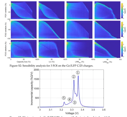
Figure S2 presents an example of the sensibility of 3 FOIs for capacity loss, LLI, LAMPE, and

527

LAMNE. The three selected FOIs were the capacity of the first plateau (area under peak ① on Figure

528

S3), the capacity of everything but the first plateau (area under peaks ②-⑤), and the capacity of the

529

last plateau (area under peak ⑤) [20]. As reported in our previous work, [20], the sensibility

530

analysis showcase that no single FOI can track capacity loss nor one of the degradation modes alone

531

since there is always a spread of values. Nonetheless, as reported in [20], their combined variations

532

might be used. This will be discussed in supplementary note 2.

533

534

535

Figure S2: Sensibility analysis for 3 FOI on the Gr//LFP C/25 charges.

536

537

Figure S3: IC signature of a Gr//LFP C/25 charge with the typical peak indexed 1-5.

538

Supplementary Note 2: Prognosis Dataset Analysis

540

The prognosis dataset can be used to test the validity of different FOIs proposed in the literature

541

for early prognosis. Figure S4 (a,b) presents the evolution of the variance between cycle one and

542

cycle 100 and 500 respectively as a function of cycle life, defined as the cycle at which 20% capacity

543

loss is reached. When considering a multitude of degradation paths, the variance approach seems

544

less effective than proposed in the literature [5,11] with correlation coefficients of -0.56 and -0.43,

545

respectively, when calculated after 100 and 500 cycles. Looking at the capacity loss after 100 cycles,

546

Figure S4 (c), the correlation is better (ρ = 0.63). Still, the error could be huge for low capacity loss as

547

paths with less than 1% capacity loss after 100 cycles were found to induce 20% capacity loss after

548

just 200 cycles. Finally, as predicted [20,21], the evolution of the first LFP plateau capacity (i.e., the

549

area under peak ① in the Gr//LFP IC curves) is not a good indicator with a Pearson coefficient of

550

0.51, Figure S4(d). The dataset could be analyzed further by tracking if specific conditions exist

551

where the FOI is accurate, e.g., the first LFP plateau capacity is likely working well when there is

552

little LAMNE [20,21]. This is out of the scope of this publication and will be investigated in future

553

work.

554

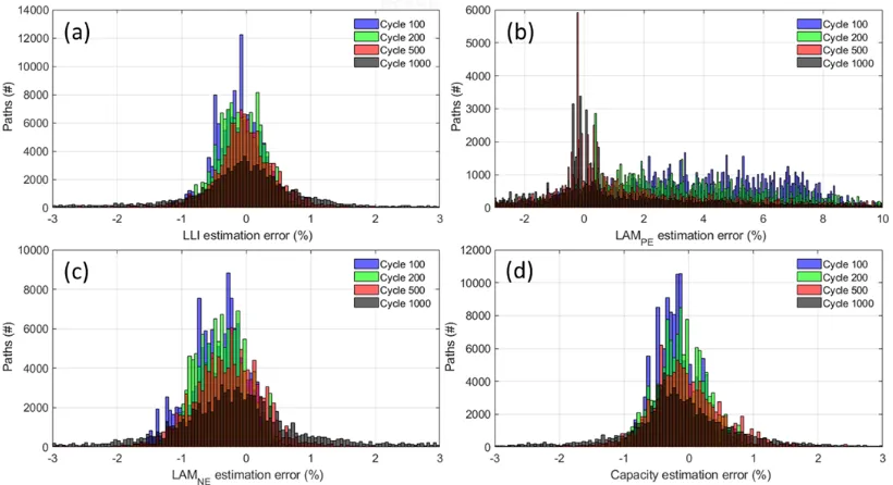
The prognosis dataset can also be used to validate diagnosis techniques. For example, the

555

method proposed in [20] can be tested. As shown in Figure S2 individual FOI information is not

556

enough to reach a proper diagnosis, but their combined variations might be enough. Figure S5

557

presents the diagnosis results based on the combined variations of 3 FOIs for diagnosis after 100,

558

200, 500, and 1,000 cycles for the 130,000 computed duty cycles. Out of the more than 500,000 points

559

tested (4 x 130,000), the average errors for estimation of LLI, LAMPE, LAMNE, and capacity loss were

560

of -0.32%, -2.73%, -0,46%, and -0.33% respectively with standard deviations below 1% for all but

561

LAMPE (6%) for diagnosis up to the 500th _{cycle. The distribution of the results is presented in Figure}

562

S5 and the different statistics summarized in Table S2. For all, but LAMPE, most of the errors are

563

comprised between -1 and 1%, with the minimum average error recorded for the diagnosis after 500

564

cycles and the maximum for the diagnosis after 1,000 cycles. The spread for LAMPE is larger,

565

between -2 and 10%, which was expected since LAMPE is notoriously hard to quantify for LFP cells

566

because of the single voltage plateau [25]. The average LAMPE error decreased with cycle number to

567

0.74% after 1,000 cycles. Looking more into details, the maximum and minimum errors were always

568

recorded for the diagnosis at 1,000 cycles with maximum and minimum errors mostly below 10% for

569

all the other cycles (except for LAMPE). Future work will investigate the specific combinations that

570

led to large errors, although our previous work [20] showed that it was for degradations unlikely to

571

happen under real-life conditions where LLI usually predominates.

572

584

Figure S4: Evolution of the (a) the variance between cycle 100 and 1, (b) the variance between

585

cycle 500 and 1, (c) the capacity loss at cycle 100 and (d) the area of the high voltage IC peak at cycle

586

100 as a function of cycle life (i.e., cycle at which 20% capacity loss is reached).

587

588

589

590

Figure S5 Distribution of the estimation errors for (a) LLI, (b) LAMPE, (c) LAMNE, and (d) the

591

capacity loss based on the evolution of 3 FOIs at cycle 100, 200, 400, and 1000.

592

593

594

595

596

597

598

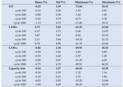
Table S2: Main error with standard deviation as well as minimum and maximum error for the three

600

degradation modes and the capacity loss.

601

Mean (%) Std (%) Minimum (%) Maximum (%)

LLI -0.32 2.39 -71.86 39.31

cycle 100 -0.12 0.34 -1.53 0.87

cycle 200 -0.08 0.36 -1.42 1.45

cycle 500 -0.02 0.79 -8.73 9.39

cycle 1000 -1.13 4.75 -71.86 39.31

LAMPE 2.73 5.82 -61.35 63.60

cycle 100 4.17 2.71 -3.66 13.07

cycle 200 3.47 3.47 -8.82 21.05

cycle 500 2.31 5.84 -34.10 41.15

cycle 1000 0.74 8.98 -61.35 63.60

LAMNE -0.46 2.36 -49.91 46.52

cycle 100 -0.45 0.42 -1.65 0.85

cycle 200 -0.39 0.40 -1.97 1.00

cycle 500 -0.28 0.67 -11.49 4.28

cycle 1000 -0.75 4.78 -49.91 46.52

Capacity loss -0.33 2.37 -60.43 43.29

cycle 100 -0.18 0.35 -1.32 1.16

cycle 200 -0.10 0.41 -1.51 1.86

cycle 500 -0.03 0.92 -10.20 10.68

cycle 1000 -1.04 4.69 -60.43 43.29

602

The results from Figure S4 raise the important question of whether a single point early

603

prognosis is possible. With the diagnosis approach validated, a possible solution could be to use

604

different diagnoses and extrapolate the evolution of the different parameters to reconstruct the

605

voltage curves using the mechanistic approach, Figure S6. This technique is already used to forecast

606

the evolution of capacity loss for large experimental studies [59,61,66]. Further work is in progress to

607

affine the technique further and to understand under which conditions the estimation is the most

608

accurate.

609

610

611

Figure S6: (a) Schematic representation of possible early prognosis solution using the

612

mechanistic approach.

613