Transfer-Efficient Face Routing Using the Planar
Graphs of Neighbors in High Density WSNs
Eun-Seok Cho1,2,†,‡, Yongbin Yim1and Sang-Ha Kim1,*
1 Department of Computer Science and Engineering, Chungnam National University, Daejeon, Korea;
[email protected] (E-S.C.); [email protected] (Y.Y.)
2 Information Technology Management Division, Agency for Defense Development, Daejeon, Korea;
* Correspondence: [email protected]; Tel.: +82-42-821-6271 † Current address: [34186] P.O.Box 35, Yuseong, Daejeon, Korea ‡ These authors contributed equally to this work.
Abstract: Face routing has been adopted in wireless sensor networks (WSNs) where topological 1
changes occur frequently or maintaining full network information is difficult. For message forwarding 2
in networks, a planar graph is used to prevent looping, and because long edges are removed by 3
planarization and the resulting planar graph is composed of short edges, messages are forwarded 4
along multiple nodes connected by them even though they can be forwarded directly. To solve this, 5
face routing using information on all nodes within 2-hop range was adopted to forward messages 6
directly to the farthest node within radio range. However, as the density of the nodes increases, 7
network performance plunges because message transfer nodes receive and process increased node 8
information. To deal with this problem, we propose a new face routing using the planar graphs 9
of neighboring nodes to improve transfer efficiency. It forwards a message directly to the farthest 10
neighbor and reduces loads and processing time by distributing network graph construction and 11
planarization to the neighbors. It also decreases the amount of location information to be transmitted 12
by sending information on the planar graph nodes rather than on all neighboring nodes. Simulation 13
results show that it significantly improves transfer efficiency. 14
Keywords:face routing; distributed processing; planar graph; transfer efficiency; high density WSN 15
1. Introduction 16
Wireless sensor network (WSN) is a multi-hop wireless network composed of a number of 17
randomly deployed sensors capable of communicating for a specific purpose. For data delivery 18
in WSNs, geographic routing has been considered as an appropriate routing strategy due to 19
being stateless under the constrained resources and a number of data transferring methods using 20
geographic information in WSNs have been studied [1–4]. Geographic routing using the location 21
information of a node instead of its network address has been classified as single-path, multi-path, 22
and flooding-based [5]. Greedy routing and face routing are used in the single-path approach. 23
Greedy routing forwards a message to a neighbor node closest to the destination, but routing 24
fails if there is no neighbor node closer to the destination than the message transfer node. However, 25
face routing transmits a message along the face boundary of a planar graph built by eliminating 26
intersecting edges that can cause loops in a network graph. It is used as one of the methods for 27
handling communications in a void area where a message cannot be forwarded by greedy routing [6]. 28
Face routing involves a planarization process which removes intersecting edges in a network 29
graph in order to construct a planar graph, whereby the generated planar graph should not be 30
segmented due to the eliminated edges. The Gabriel graph (GG) [7] and the relative neighborhood 31
graph (RNG) [8] are representative planar graphs in which the network is not cut off when they are 32
constructed using only local information [9]. In order to perform planarization while preventing the 33
segmentation of a network, GG and RNG remove long edges that might be an intersecting edge in 34
a network graph. Therefore, planarization results in a planar graph consisting of only short edges. 35
However, this causes inefficiency because a message is sequentially transferred to the remote node 36
within radio range along the nodes on a face boundary made up of short edges even though it could 37
be directly forwarded. 38
In order to mitigate the inefficiency, face routing using the location information on all nodes 39
within 2-hop range has been proposed [10]. It forwards a message directly to the most remote neighbor 40
located on the routing path within radio range. In this method, a message transfer node builds a local 41
full network graph within radio range using 1- and 2-hop node information, performs planarization 42
to construct a local full planar graph within radio range, discovers the most remote node to which a 43
message can be forwarded, and sends a message directly to the selected node without traveling via 44
intermediate nodes. Since the location information on all the 2-hop nodes as well as the immediate 45
neighboring nodes must be transmitted to the message transfer node, the amount of information to be 46
transmitted is increased compared to legacy face routing. In addition, because the method requires 47
construction of a network graph using the increased information and then performing planarization, 48
the number of calculations is increased, as is the consumption of resources such as memory and energy. 49
This phenomenon makes the efficiency drop sharply due to the long computation time and the 50
high energy consumption caused by the large number of nodes deployed within radio range and 51
their position information in a high density WSN. In addition, whenever a node within 2-hop range is 52
added or deleted and regardless of whether it affects the routing, the message transfer node always 53
receives information on the changed node and performs network graph generation, planarization, and 54
routing again. 55
In this paper, we propose a novel face routing that uses the planar graphs of the message transfer 56
node’s neighbors to forward a message to the most remote neighbor on the route within radio range 57
without traveling via intermediate nodes to improve transfer efficiency and to solve the problems 58
previously mentioned in existing face routing methods. 59
In the proposed face routing, a message transfer node receives the information on the planar graph 60
of its neighbors and it constructs a local full planar graph within radio range. Using the generated 61
planar graph, the most remote neighbor node on a routing path is discovered and the message is 62
transferred directly to the node without traveling via intermediate nodes. Unlike face routing using 63
2-hop node information, the load for generating the local planar graph is distributed to each neighbor, 64
which reduces the amount of location information to be transmitted by sending only the information 65
on the planar graph nodes rather than on all of the neighboring nodes. In addition, the efficiency 66
can be improved by virtue of only receiving information when a node changes and recalculating the 67
routing if there is an influence on the planar graph rather than every time a node is added or destroyed. 68
That is to say, if a node is added to the network but it is removed during the planarization process 69
of the neighbor, the changed node information need not be transmitted to the message transfer node 70
and it is not necessary to recalculate the routing. And, if a node is removed from the network but 71
has already been deleted in the existing planar graph, the changed topology need not be transmitted. 72
Furthermore, in order to improve transfer efficiency while balancing energy consumption of each node, 73
a message transfer node, if its remaining power is low, sends a message to the nearest neighbor along 74
a face boundary instead of forwarding it to the remote node to minimize energy consumption. 75
The rest of the paper is organized as follows. In Section2, we provide a review of related work. 76
In Section3, we discuss the problem of planar graphs and planarization, and in Section4, we explain 77
the proposed face routing in detail. In Section5, a comparison of its performance with existing 78
researches through experiments is reported, and conclusions are drawn in Section6. 79
2. Related Works 80
Early proposals for face routing methods using planar graphs include Greedy Face 81
Greedy Other Adaptive Face Routing (GOAFR+) [13], GOAFR++ [14], and Greedy Path Vector Face 83
Routing (GPVFR) [15]. The methods forward a message along a sequence of faces intersecting with 84
line stbetween the source (s) and the destination (t). A face change occurs when the edge of a 85
face intersects with linest. Messages are delivered based solely on local information and the faces 86
are traversed sequentially, and to improve performance, they are able to choose whether to pass 87
through the intersecting edge or not when changing the face or to change how linestis set up and 88
used. That is to say, they improve performance by changing the face after going through or without 89
passing through the intersecting edge. They also enhance efficiency by using the initial setup of linest 90
without changing during the entire routing process, or using a newly set up linestwhenever a face is 91
changed. Their performance also depends on the choice of traversal direction change, i.e. clockwise or 92
counterclockwise. In short, early face routing improves performance and efficiency by determining 93
how linestis set, when to change the face, which face to change to, and in which direction to explore 94
the face is. 95
ProgressFace [16] and Concurrent Face Routing (CFR) [17] have improved the performance and 96
efficiency of early face routing by modifying how to forward the message instead of adjusting how 97
to change the face. ProgressFace alleviates the problem of too many hops being taken if messages 98
are forwarded in the wrong direction due to the unbalanced deployment of the nodes. It finds the 99
direction with the smallest number of hops through an additional traversal step and improves routing 100
efficiency by setting the forwarding direction to the way it finds, after which it sends the message. 101
CFR focuses on the speed of message delivery and accelerates the message propagation by sending 102
messages concurrently in both directions of faces intersecting with linest. It can send messages to the 103
destination via the shortest possible route because it disseminates them through all available routes via 104
the faces adjacent to linest. Although it sends many duplicate messages to the network, it improves 105
routing performance by sending messages at speeds similar to those sent by the shortest path. 106
All of these face routing methods have improved the performance, efficiency, and speed of routing 107
by selecting the face, enabling changes of the face if necessary, adjusting the search direction, and using 108
an additional traversal step or forwarding duplicate messages. However, since they forward messages 109
by sequentially exploring all the nodes constituting a face regardless of radio range, performance 110
rapidly deteriorates due to the increased number of nodes that need to be traversed in high density 111
WSNs. 112
In order to improve the forwarding efficiency by considering radio range, face routing using 113
all of the node information within 2 hops has been proposed [10]. This improves routing efficiency 114
by building a local full planar graph with the information of the 1- and 2-hop nodes, and directly 115
forwarding the message to the most remote node within radio range using the generated graph. 116
However, it is also unsuitable for high density WSNs due to the increased communication cost for 117
transmitting the location information of such a large number of nodes within a 2-hop range and the 118
performance degradation caused by the increased calculation cost due to the increased number of 119
nodes. 120
3. The Problem with Planar Graphs and Planarization 121
GG and RNG are representative planar graphs constructed using only local information and do 122
not divide a network. They are built by removing what might be intersecting edges among the edges 123
between a message transfer node and its neighbors. Figure1shows the process of building a local 124
GG: Figure1a represents the local network graph of nodeuand Figure1b depicts the planarization 125
process which eliminates edges that do not fit the GG edge condition. An edge is removed if there is a 126
node other than nodeuand a neighbor in the circle whose diameter is their edge. To illustrate this, in 127
Figure1b, nodeaexists in the circle within the edge diameter between nodesuandx, soedge(u,x) 128
is removed. Figure1c shows the planar graph generated after planarization. For the edge removal 129
process according to the GG edge condition, long edges are removed and only short edges are left. 130
(a) (b) (c)
Figure 1.Planarization process: (a) local full network graph (r: radio range), (b) planarization, and (c) local Gabriel graph (GG).
(a) (b)
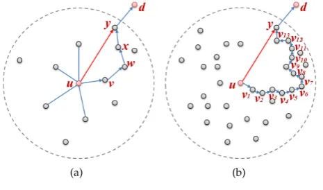
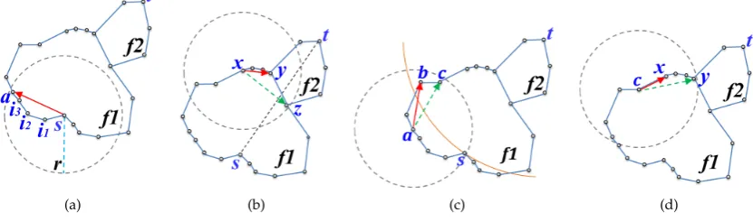
Figure 2.Face routing according to the node density: (a) a low density network, and (b) a high density network.
message sequentially along multiple nodes in the face in spite of being able to send it directly when in 132
radio range. 133
In Figure2a, if nodesu,v,w,x,y, anddare on the routing path that make up the face, a problem 134
with efficiency arises in that a message should have been transferred to nodeyafter exploring nodes 135
v,w, andx, but becauseedge(u,y)was removed during planarization, the message cannot be forwarded 136
from nodeudirectly to nodey. Consequently, in a high density WSN, the inefficiency caused by 137
this becomes even more exacerbated, as shown in Figure 2b; a message is transmitted through 138
15 hops (u→v1→...→v13 →y→d) even though it could be transferred in only 2 hops (u→y→d).
139
As the density of the nodes increases, the number of nodes within radio range increases, and as this 140
happens, the edges of the planar graph become shorter during planarization. The shortened edges 141
intensify the inefficiency because they increase the number of nodes that need to be traversed when 142
forwarding a message. 143
4. Transfer-Efficient Face Routing 144
In this section, we explain in detail the proposed face routing: transfer-efficient face routing 145
(TEFR), which improves transfer efficiency by using the planar graph of the neighbor. We describe the 146
exchange of location information between nodes and the construction of local planar graphs, then we 147
define the process of discovering the node to send a message to using the generated planar graphs of 148
its neighbors. Finally, we analyze the performance of the proposed face routing. 149
TEFR is used in conjunction with greedy routing for message forwarding in void areas where 150
two-dimensional plane, that the link between nodes is reliable, and that their power status, their own 152
position and the location of the source and destination of the message are known. We used a GG 153
composed of a unit disk graph as a planar graph. 154
4.1. The Exchange of Location Information 155
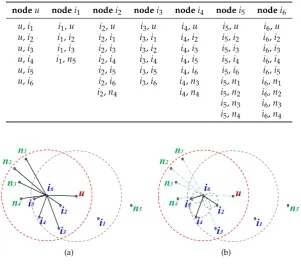
The first step of TEFR is to exchange location information between nodes. Since TEFR is a 156
position-based routing method, it is necessary to collect the location information of the neighbors 157
that is exchanged periodically using a beacon or aperiodically when there are topological changes. A 158
beacon message consists of three fields: 159
• id: the local identifier of a node used to distinguish nodes within 2-hop range. 160
• LxandLy: thexandycoordinates of a node indicating its location. 161
Since the message transfer node in TEFR uses the planar graph of itself and its neighbors, it can 162
receive position information on 2-hop nodes from its neighbors. Therefore, all nodeids should be 163
identified within 2-hop range. Figure3demonstrates the exchange of location information between 164
nodes. Since message transfer nodeucan receive location information onn1,n2,n3,n4, andn5located
165
at 2 hops from neighbors,i1,i2,i3,i4,i5, andi6, nodeids need to be distinguished within 2-hop range.
166
Figure 3.Beaconing: the exchange of position information between nodes.
4.2. Build a Local Planar Graph 167
The second step of TEFR is to construct a local planar graph using the location information on the 168
neighboring nodes and to transfer the information on the constructed planar graph to the message 169
transfer node. The message transfer node and its neighbors generate their own local network graphs 170
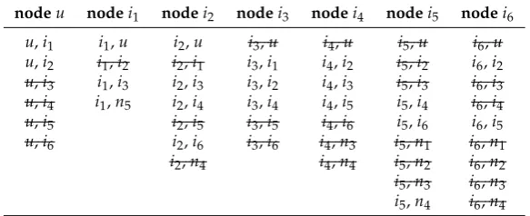
and their local GGs are built after planarization. Table1shows the edge list of the constructed local 171
network graph of the message transfer node and its neighbors after exchanging location information 172
between nodes in the network in Figure3. Although the local network graph is part of the overall 173
network graph, it is still possible to cause a loop across the entire network. Thus, even though the local 174
network is tiny, it is necessary to remove any intersecting edges which might cause a loop by applying 175
planarization. 176
A local GG edge list is built for the message transfer node and its neighbors by removing edges 177
that do not satisfy the GG edge condition from the edge list of the local network graphs to prevent 178
looping. Figure4shows a local network graph and a local planar graph of nodei6as an example of a
179
planar graph built for the neighbors of a message transfer node. In Figure4a, to perform planarization 180
for nodei6, the GG edge condition is applied to all the edges connected to its neighbors. The resulting
181
Table 1.The local network graph edge lists of message transfer nodeuand its neighbors in Figure3.
nodeu nodei1 nodei2 nodei3 nodei4 nodei5 nodei6
u,i1 i1,u i2,u i3,u i4,u i5,u i6,u
u,i2 i1,i2 i2,i1 i3,i1 i4,i2 i5,i2 i6,i2
u,i3 i1,i3 i2,i3 i3,i2 i4,i3 i5,i3 i6,i3
u,i4 i1,n5 i2,i4 i3,i4 i4,i5 i5,i4 i6,i4
u,i5 i2,i5 i3,i5 i4,i6 i5,i6 i6,i5
u,i6 i2,i6 i3,i6 i4,n3 i5,n1 i6,n1
i2,n4 i4,n4 i5,n2 i6,n2
i5,n3 i6,n3
i5,n4 i6,n4
(a) (b)
Figure 4.Local graphs of nodei6: (a) the local network graph, and (b) the local Gabriel graph (GG).
Planarization is performed independently on the message transfer node and all its neighbors. 183
The pseudo-code running on each node for generating the GG edge list from the edge list of a local 184
network graph is as follows. 185
Algorithm 1Generating the GG edge list from the edge list of a local network graph. LNG: edge list of the local network graph
LGG: edge list of the local Gabriel graph forall edges inLNGdo
if(there exists no node in the circle with edge’s diameter)then add edge toLGG
end if end for
The algorithm generates the GG edge list by selecting those edges meeting the GG edge condition 186
among all edges on the local network graph. Table2shows the GG edge lists constructed by applying 187
Algorithm1to the local network graph edge lists in Table1. The strikethroughs in Table2represent 188
Table 2.The local planar graph edge lists of nodeuand its neighbors in Figure3.
nodeu nodei1 nodei2 nodei3 nodei4 nodei5 nodei6
u,i1 i1,u i2,u i3,u i4,u i5,u i6,u
u,i2 i1,i2 i2,i1 i3,i1 i4,i2 i5,i2 i6,i2
u,i3 i1,i3 i2,i3 i3,i2 i4,i3 i5,i3 i6,i3
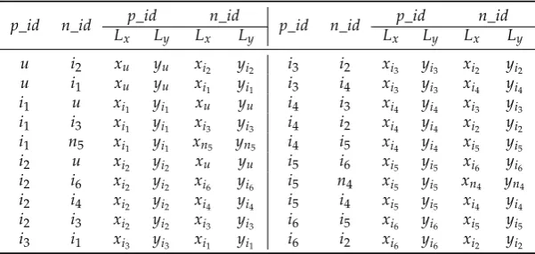
u,i4 i1,n5 i2,i4 i3,i4 i4,i5 i5,i4 i6,i4
u,i5 i2,i5 i3,i5 i4,i6 i5,i6 i6,i5
u,i6 i2,i6 i3,i6 i4,n3 i5,n1 i6,n1
i2,n4 i4,n4 i5,n2 i6,n2
i5,n3 i6,n3
i5,n4 i6,n4
Since TEFR distributes planarization to the neighbors of the message transfer nodes, it is possible 190
to solve the problem that the load is concentrated on the message transfer nodes, which makes face 191
routing using 2-hop node information so inefficient. Moreover, because a message transfer node only 192
receives information of the planar graph nodes rather than of all neighboring nodes, the amount of 193
position information to be transmitted can be reduced. In addition, the changes are transmitted to a 194
message transfer node each time a node is added or removed only if the planar graph is affected due 195
to a change in topology. Therefore, TEFR improves efficiency and minimizes the amount of location 196
information that needs to be transferred. 197
(a) (b)
Figure 5.Topological changes that do not affect the planar graph: (a) changed local network graph, and (b) (a)’s planar graph.
(a) (b)
Figure 6. Topological changes that affect the planar graph: (a) changed local network graph, and (b) (a)’s planar graph.
Figure5and Figure6show two cases where the changed node information is either sent or not 198
topology is changed but the changes do not affect the planar graph, while Figure6shows the opposite 200
case to Figure5where the changed node information should be sent to the message transfer node. 201
Figure5a is the local network where new nodesa1anda2are added, and nodei3is deleted in the
202
network of Figure4a. Even if nodesa1anda2are added but the edges between nodei6and them are
203
deleted during planarization, this does not affect the existing planar graph. Furthermore, even though 204
nodei3is removed from the network sinceedge(i6,i3)has already been deleted from the existing
205
planar graph due to not fitting the GG edge condition, this also does not affect the existing planar 206
graph. Figure5b shows the planar graph after topological changes have occurred. Since it is the same 207
as before the network change, the changed node information is not transmitted even though there 208
have been topological changes. 209
Figure6shows the case where a topological change affects the planar graph. Figure6a depicts the 210
local network where new nodeb1is added to the network of Figure4a andi4is deleted.edge(i6,b1)
211
becomes a new edge on the planar graph according to the GG edge condition, andedge(i6,i4), which
212
was an edge on the existing planar graph, is removed because the node has been deleted (Figure6b 213
shows the planar graph after adding and removing the nodes). Since the existing planar graph has 214
been changed, the changed planar graph information on nodei6must be sent to the message transfer
215
node. 216
4.3. Remote Node Selection and Message Forwarding 217
The last step in the TEFR is to discover the node located at the most distant hop on a routing 218
path within radio range using the information on the planar graphs of the neighbors at the message 219
transfer node, and then send the message. The message transfer node generates an edge list of the full 220
planar graph within radio range using the local planar graph information received from the neighbor 221
to determine which node the message is to be transferred to. 222
Table3shows the full GG edge list within radio range built with the planar graph information 223
of its neighbors at message transfer nodeuin Figure3. Each item in the edge list consists of the start 224
nodeid, the end nodeid, and theirx,ycoordinates: p_id, the immediate neighbor of the message 225
transfer node, is the nodeidwhose local planar graph is sent to the message transfer node and is the 226
starting node of the edge;n_idrepresents the opposite side node of the edge; andLxandLyrepresent 227
the location information for thep_idandn_idnodes. When the start and end nodes of all edges in 228
the list are connected, a full planar graph within radio range of a message transfer node is generated. 229
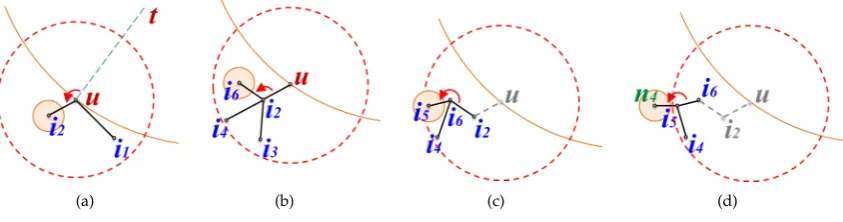
Figure7shows the local full GG within radio range of message transfer nodeu, which is constructed 230
using the edges in Table3. 231
TEFR uses the generated edge list to determine the node to send the message to. In the discovery 232
process, four cases need to be considered, as shown in Figure8. The first three cases are for direct 233
forwarding to the remote node within radio range and the last case is for sequential forwarding applied 234
Table 3.The GG full edge list of nodeuwithin radio range in Figure3.
p_id n_id p_id n_id p_id n_id p_id n_id Lx Ly Lx Ly Lx Ly Lx Ly
Figure 7.Local full Gabriel graph (GG) within radio range of nodeu.
when the remaining power of a message transfer node is insufficient. For direct transmission, the first 235
is when message forwarding occurs within the same face, the second is when a face change occurs, 236
and the third is when the routing mode is switched from face routing to greedy routing. 237
In the first case, a message is sequentially transferred along the face within radio range and the 238
change of face or routing mode does not occur during the routing. In this instance, the node located at 239
the last hop of the face boundary within radio range is selected as the node where the message is to be 240
sent to. Figure8a shows the case where a message is forwarded within the same face. TEFR selects 241
nodealocated at the farthest hop within radio range of message transfer nodesas the most remote 242
node, and the message is sent to it. 243
The second case arises when a face change occurs while the message is forwarded within radio 244
range because the line from the source to the destination and a face boundary edge intersect. In this 245
case, TEFR transmits a message to the node where the intersecting line occurs, not the most distant 246
hop node within radio range. After the selected node receives the message, it changes the face and 247
routing is continued. Figure8b shows the case where the face is changed because the intersection 248
between linestandedge(y,z)occurs while traveling to the face within radio range of message transfer 249
nodex. If a message is sent to the most distant nodezwithout considering the face change at message 250
transfer nodex, a loop occurs because the face change does not execute. Therefore, message transfer 251
nodexforwards the message to nodeywhere the face change occurs, after which nodeychanges the 252
face and then continues routing. 253
The third case happens when it is necessary to switch to greedy routing while traveling to a face 254
within radio range. TEFR immediately switches from face routing to greedy routing when greedy 255
(a) (b) (c) (d)
routing is enabled and it forwards a message according to greedy routing. Figure8c shows the case 256
where the routing mode needs to be switched from face routing to greedy routing during face traversal 257
within radio range. Message transfer nodeaforwards a message to the first nodebcloser to the 258
destination (t) than nodeswhere face routing started without sending a message to the farthest hop 259
nodecon the face boundary within radio range. After receiving the message, nodebswitches to 260
greedy routing and performs message forwarding. 261
The last case occurs when a message transfer node has low residual power. A message is sent 262
sequentially along a face boundary instead of being forwarded to the remote node. Because energy 263
consumption increases as the distance to be transmitted increases in wireless communication [18], a 264
message transfer node sends a message to its nearest neighbor when the energy level is low to minimize 265
power consumption. This extends the lifetime of the node and consequently prolongs the lifetime 266
of the WSN. By selectively transmitting a message to the remote node or nearby nodes according to 267
the remaining power, transfer efficiency can be improved while using the energy of each node in a 268
balanced manner. Figure8d shows the case where a message transfer node has less energy than the 269
threshold for direct transmission. Message transfer nodeccan forward a message directly to remote 270
nodey, but it sends a message to nearest nodexto minimize energy consumption. 271
Since TEFR can determine the routing path in advance within radio range using the full GG edge 272
list, it can establish the most remote node where a message can be transferred most efficiently, and a 273
message can be sent directly to the selected node. That is to say, TEFR can directly send a message 274
without journeying via intermediate nodes by simulating routing internally using the edge list as in 275
Table3and selecting a remote node in the same way as actually traveling the nodes constituting the 276
face within radio range. 277
Figure9shows the internal process of node selection at a message transfer node required to send 278
a message, which corresponds to the case of forwarding a message within the same face as in Figure8a. 279
All the processes in Figure9are performed internally at message transfer nodeu, and after the process 280
is finished, a message is forwarded to the selected node. 281
Figure9a shows the beginning of the face routing simulation to establish the node where the 282
message is to be sent to. Face routing is started at message transfer nodeubecause there is no node 283
closer than itself to the destination (t) among the neighbors. Nodeuselectsi2as the next node to be
284
explored by applying the left-hand rule based on lineutamong neighboring nodesi1andi2in the GG
285
edge list in Table3. 286
In Figure9b, nodei2selectsi6as the next node to explore according to the left-hand rule, and
287
checks whether it is within radio range of nodeu, whether the routing mode should be switched to 288
greedy routing, and whether an intersecting edge occurs. Nodei6is located within radio range of
289
nodeu, is farther from the destination than nodeuwhere face routing started, andedge(i2,i6)does not
290
(a) (b) (c) (d)
Figure 9.Phases of TEFR node selection: (a) the start of simulating face routing, (b) & (c) select the next nodes of nodesi2andi6, respectively, and (d) the termination of node selection. The arc signifies
intersect lineut. Thus,i6is selected as the next node to navigate to. In Figure9c,i5is selected as the
291
next node to travel to from nodei6in the face routing procedure according to the same condition as
292
nodei6.
293
In Figure9d, noden4, which is the next node along from nodei5, is beyond the radio range of
294
message transfer nodeu. Therefore, message transfer nodeuterminates the node discovery process 295
and selectsi5as the target node to send the message to. Message transfer nodeuimproves the transfer
296
efficiency by sending a message directly to the most remote nodei5without actually passing through
297
the intermediate nodesi2andi6. The pseudo-code for selecting the most remote node using the GG
298
full edge list of a message transfer node and sending a message is as Algorithm2. 299
Algorithm 2Selecting the most remote node using the GG edge list and sending a message.
lhn: a node according to left hand rule ctn: a current traversal node
mtn: a message transfer node
f rn: a node where face routing started
thd: the power threshold for direct transmission selectlhnofctnfrom GG edge list
if( the power level ofctn<thd) then send message tolhn, exit
end if
while(lhnis located within radio range ofmtn)do if(lhnis closer to the destination than f rn)then
change mode to greedy routing send message tolhn, exit
else if(the edge betweenlhnandctnintersectsst)then send message toctn, exit
else
setctnwithlhn
selectlhnofctnfrom GG edge list end if
end while
send message toctn, exit
4.4. Analysis 300
TEFR utilizing the local planar graphs of the message transfer node’s neighbors needs more location information compared with legacy face routing using local information but uses less position information than face routing using the information on all nodes within 2-hop range. Equation (1) compares the quantity of location information transmitted to a message transfer node. In the equation, the left hand side is legacy face routing, the middle is TEFR, and the right hand side is face routing using 2-hop node information:
n×m≤n×m+n×((1−λ)×n)×m≤n×m+n2×m, (1) wherenis the average number of neighboring nodes per node,mis the data size of location information 301
for one node, andλis the ratio of nodes removed in planarization (0≤λ<1). 302
In equation (1), in legacy face routing, a message transfer node only receives location information 303
on the average number of neighboring nodes, while TEFR receives the location information on the 304
immediate neighbors and their planar graph nodes after planarization. Face routing using 2-hop node 305
well. The amount of location information required for TEFR is the same as that for face routing using 307
2-hop node information when nodes are not removed in the planarization step (λ= 0), and becomes 308
close to that of legacy face routing as the number of removed nodes increases. 309
In a high density WSN, TEFR does not rapidly increase the amount of position information to be 310
transmitted because even if the number of nodes increases, those removed by planarization increases 311
andλbecomes bigger as the density of the nodes increases. TEFR uses the location information on 312
more nodes than the legacy face routing to improve transfer efficiency, but it reduces the amount of 313
position information in comparison with face routing using 2-hop node information because message 314
transfer nodes only receive the information on the planar graph nodes of their neighbors. 315
Equation (2) compares the end-to-end delay of face routing within radio range. The first formula is the delay of legacy face routing, the second is that of face routing using 2-hop node information, and the last is that of TEFR.
(n−1)×(Dew+Dt+k×Dpp+Dps+Dq), Dew+Dt+k2×Dpp+Dps+Dq
≥Dew+Dt+k×Dpp+Dps+Dq. (2) End-to-end delay can be divided into propagation delay (Dew), transmission delay (Dt), processing 316
delay (Dp), and queueing delay (Dq) [19]; we divide Dp into the time (Dpp) required to execute 317
planarization for individual neighboring nodes and the time (Dps) for determining the node to which 318
the message is to be sent. Furthermore, in the formulae,nis the number of nodes on the face boundary 319
to be traveled within radio range (n>1) andkrepresents the average number of neighboring nodes. 320
In equation (2), since legacy face routing needs to sequentially travel the nodes on the face 321
boundary, the end-to-end delay is highly influenced by the number of nodes constituting the face. 322
However, TEFR and face routing using 2-hop node information are not affected by the number of 323
nodes constituting the face because the message is forwarded directly to the most remote node within 324
radio range. 325
Since face routing using 2-hop node information performs planarization on all edges within 2-hop 326
range of the message transfer node, the execution time of planarization is required for the square 327
of the number of neighboring nodes. On the other hand, TEFR only requires the execution time for 328
planarization on the local nodes because it performs planarization independently on each neighboring 329
node. As the number of deployed nodes increases, the performance of face routing using 2-hop 330
node information decreases rapidly due to the increase in planarization time caused by squaring the 331
number of neighboring nodes. In contrast, TEFR can forward a message without an abrupt decrease in 332
performance because the planarization time is gradually prolonged in proportion to the number of 333
neighboring nodes. 334
5. Performance Evaluation 335
In this section we compare the performance of legacy face routing, face routing using 2-hop 336
node information, and the face routing proposed in this paper. In order to compare the independent 337
performance of each, we implemented the simulation with only face routing except greedy routing. 338
5.1. Simulation Environment 339
We simulated the performance of the proposed face routing using the network simulator Qualnet 340
4.0 [20]. The radio range of the sensor node was 50∼250m, and 200∼1,500 nodes were randomly 341
deployed in a space of 1,000 x 1,000m2. The network model was a unit disk graph connected from the 342
source to the destination, and GG was used as the planar graph. The simulation time was set to 100 343
seconds and each sensor node transmitted its position to its neighbors. All the results were the average 344
of each simulation experiment repeated 100 times. In the simulation, Greedy Face Greedy Routing 345
using all node information within 2-hop range, and TEFR using the planar graphs of neighbors were 347
used. 348
5.2. Simulation Results 349
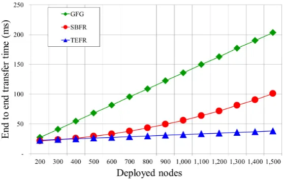
Figure10shows a graph comparing the time at which the message was forwarded from the 350
source to the destination according to the number of deployed nodes. With GFG, as the number 351
of deployed nodes increases, the number of nodes to be traveled increases because the number of 352
nodes constituting a face increases. Thereby, the transfer time increases gradually in proportion to the 353
increased number of nodes. With SBFR, since a message is sent directly to the most remote node within 354
radio range, even if the number of nodes increases, the time for forwarding a message is constant. 355
However, since it performs planarization on all nodes within 2-hop range of a message transfer node, 356
as the number of nodes increased, the computation time increased, resulting in the message transfer 357
time, which includes the computation time, becoming longer. Since TEFR sends a message directly to 358
the most remote node within radio range and the generation of the planar graph is performed in a 359
distributed manner at the neighbor node, the increase in the number of nodes has little effect on the 360
transfer time. From the experimental results, we can confirmed that the transfer time of TEFR was 361
hardly affected by an increase in the number of nodes. 362
Figure 10.Transfer time according to the number of deployed nodes (Radio range: 100m).
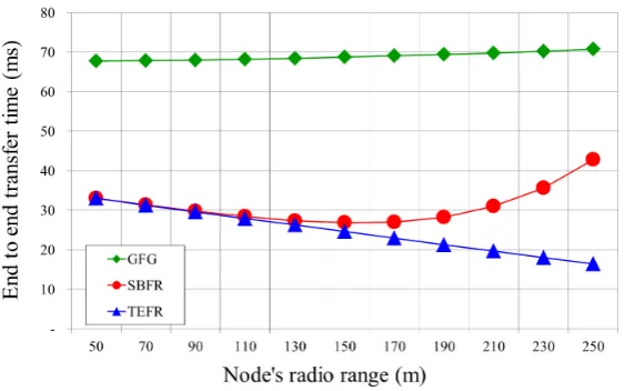
Figure11shows a graph comparing the transfer time from the source to the destination according 363
to changes in radio range. With GFG, even if the radio range is widened, it is necessary to sequentially 364
travel along the nodes connected with short edges regardless of the radio range. Thus, the transfer 365
time did not decrease even when the radio range was expanded. With SBFR, as the radio range 366
increases, a message can be directly sent to a node located at a longer distance, thereby reducing 367
the transfer time. However, as the radio range is widened, the number of nodes within radio range 368
increases and the construction time of the planar graph increases accordingly. As the radio range 369
exceeds a certain distance, the wider the radio range, the longer the transfer time. With TEFR, even if 370
the number of nodes to be planarized increases due to an increment in radio range, the transfer time is 371
not significantly affected because planarization is distributed to the neighbors of the message transfer 372
node, and the message can also be sent directly to the node farthest away. As a result, as the radio 373
range increased, the transfer time decreased. 374
Figure12shows the transfer time of each face routing according to the ratio of the node that can 375
forward a message directly to the remote node in an experiment to consider the power state of the 376
node. In practice, SBFR does not take into account the power state of the node, but in order to compare 377
Figure 11.Transfer time according to radio range (Deployed nodes: 500).
has less power than the threshold. Since GFG transfers a message sequentially along a face boundary, 379
the transfer times are similar regardless of the proportion of nodes performing direct transmission. 380
However, in SBFR and TEFR, the number of nodes forwarding a message to the remote node also 381
increases as the ratio of nodes capable of direct transmission increases, resulting in a decrease in 382
end-to-end transfer time. The ratio of nodes is 0% when all of the deployed nodes send messages 383
sequentially along the face boundary, and when the ratio of nodes is 100%, all nodes are able to forward 384
messages directly to the remote node. TEFR shows performance similar to GFG or SBFR when the 385
nodes send messages sequentially. In addition, as the number of nodes capable of direct transmission 386
increases, it performs better than GFG and SBFR due to the increased ratio of forwarding a message 387
directly to the remote node and the faster computation time for routing than SBFR. 388
Figure 12.Transfer time according to ratio of nodes capable of direct transmission (Radio range: 100m, Deployed nodes: 1500).
Figure13is a graph of the total number of hops from the source to the destination by the number 389
of deployed nodes. With GFG, as the number of deployed nodes increases, the edges on the planar 390
graph become shorter. Therefore, the number of hops to journey from the source to the destination 391
increases. Since SBFR and TEFR send a message directly to the most remote node within radio range, 392
SBFR and TEFR show similar hop counts because the number of hops is not related to computation 394
time when constructing a planar graph. 395
Figure 13.Hop counts according to the number of deployed nodes (Radio range: 100m).
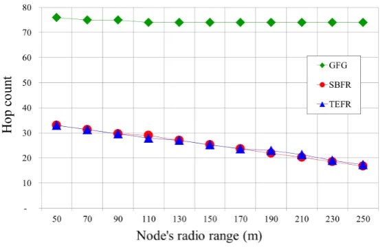
Figure14compares the number of hops with a change in radio range. With GFG, even if the node 396
that the message can be directly forwarded to is further away due to the increased radio range, since 397
long edges are removed in planarization and a message is forwarded along short edges, the radio 398
range expansion does not affect the number of hops. In SBFR and TEFR, as the radio range increases, 399
the number of hops decreases because they can transfer a message directly to a node that is further 400
away, which was confirmed by the simulation results. 401
Figure 14.Hop counts according to radio range (Deployed nodes: 500).
Figure15depicts a comparison of the amount of location information to be transmitted as the 402
number of nodes increases within the same radio range. Because GFG receives and uses only the 403
position information of the message transfer node’s neighbors, as the number of deployed nodes 404
increases, the number of neighboring nodes increases, and so the amount of the location information 405
to be transmitted gradually increases. With SBFR, since the location information on all nodes within 406
2-hop range must be transmitted to the message transfer node, the amount of location information to 407
be transmitted sharply increases as the number of nodes increases. In other words, when the average 408
Figure 15.The quantity of transferred location information according to the number of nodes (Radio range: 100m).
Figure 16.The quantity of transferred location information according to the radio range (Deployed nodes: 500).
information onn+n2nodes since it receives the location information onnimmediate neighboring 410
nodes andnneighboring nodes for each of them. With TEFR, since the position information on its 411
neighbors and their planar graph nodes is transmitted to the message transfer node, the amount of 412
position information increases further as the number of nodes increases compared to GFG. However, 413
unlike SBFR, the amount of location information does not increase rapidly because only the information 414
of the nodes after planarization is transmitted. As the number of deployed nodes increases, the number 415
of removed nodes in planarization also increases. Therefore, the amount of location information does 416
not increase sharply even if the number of nodes to be deployed increases. 417
Figure16shows changes in the amount of location information as radio range increases. With 418
GFG, as the radio range increases, the number of the neighbor increases and the amount of location 419
information to be transferred increases accordingly. With SBFR, as the radio range increases, more 420
neighboring nodes transmit position information because of the much larger number of nodes in 2-hop 421
range. Thus, as the radio range is expanded, the amount of the location information to be transmitted 422
some neighbor nodes of the planar graph after the planarization is transmitted to the message transfer 424
node, the amount of the location information is not increased by as much as with SBFR. 425
The experimental results show that the proposed face routing did not increase the transfer time, 426
unlike with GFG and SBFR, even when the number of nodes increased, and the transfer time lessened 427
as the radio range increased. A message was able to be sent to the destination within a certain number 428
of hops regardless of the number of deployed nodes as long as the network was the same size. As the 429
radio range became wider, the hop count was gradually reduced because a message can be directly 430
forwarded to a node located at a longer distance away. In comparison with face routing using local 431
information, more position information needs to be transmitted because the planar graph information 432
of the neighbor is additionally used. However, since the neighbors of the message transfer node only 433
transmit information on some nodes after planarization, it uses less location information than face 434
routing using 2-hop node information. 435
Through our experimental results, we can see that the proposed face routing was able to forward 436
a message at a faster and more constant rate in a high density WSN than the existing face routing 437
methods, and it was able to forward messages to the destination within a certain number of hops. 438
Furthermore, as the radio range was enlarged, the transfer time was reduced because the messages were 439
forwarded by traveling via a smaller number of nodes from the source to the destination. Therefore, 440
transfer efficiency can be further improved by adjusting the radio range when applying the proposed 441
face routing in practice. 442
6. Conclusions 443
In this paper, we propose a new face routing to improve transfer efficiency by forwarding a 444
message directly to the most distant hop node on a routing path within radio range using the planar 445
graphs of neighbors. Since traditional face routing transfers a message using a planar graph to prevent 446
a loop, a problem with decreased efficiency occurs as a result of forwarding a message sequentially 447
along a face boundary composed of short edges although it can be delivered directly. In order to solve 448
this problem, face routing which forwards a message directly to the most remote node within radio 449
range using all of the node information within 2-hop range has been proposed, but this makes message 450
transfer nodes receive too much location information and requires a great deal of computation for 451
network graph generation and planarization. In a high density network, it causes another problem in 452
that the processing time increases rapidly and a huge load is concentrated on the message transfer 453
nodes. 454
The proposed face routing distributes loads and reduces message transfer time by using the 455
planar graph information of the message transfer node’s neighbors. It distributes the construction 456
and planarization process of the network graph to the neighbors and reduces the amount of position 457
information to be transmitted through sending only the information concerning the planar graph 458
nodes. Furthermore, it minimizes traffic and computation time for routing by transmitting the location 459
information of changed nodes irrespective of topological changes and only when the planar graph is 460
changed. These characteristics make it suitable for use in high density WSNs. Through performance 461
evaluation, we confirmed that the proposed scheme improved transfer efficiency compared to the 462
existing face routing methods. In future research, we would like to study a method involving 463
end-to-end message forwarding within a limited timeframe regardless of the density of the deployed 464
nodes and how to efficiently forward a message in the real environment where the link is unreliable. 465
Acknowledgments: This research was supported by Basic Science Research Program through the National 466
Research Foundation of Korea(NRF) funded by the Ministry of Science and ICT(NRF-2015R1A2A2A01006442). 467
Author Contributions:Eun-Seok Cho and Yongbin Yim conceived the idea of the overall experimental strategy. 468
Eun-Seok Cho carried out the simulations and wrote the paper. Yongbin Yim supported writing and revising the 469
article. Sang-Ha Kim provided valuable feedback and supervised the work. 470
References 472
1. Santos, R.; Edwards, A.; Verduzco, A. A geographic routing algorithm for wireless sensor networks.IEEE 473
Proceedings of the Electronics, Robotics and Automotive Mechanics Conference.2006, 64-69. 474
2. Ruhrup, S. Theory and practice of geographic routing.Ad Hoc and Sensor Wireless Networks: Architectures, 475
Algorithms and Protocols.2009, 69. 476
3. Al-Karaki, J.N.; Kamal, A.E. Routing techniques in wireless sensor networks: A survey. IEEE Wireless 477
communications.2004,11, 6-28. 478
4. Seada, K.; Helmy, A. Geographic protocols in sensor networks.ASP Encyclopedia of Sensors.2004. 479
5. Stojmenovic, I. Position-based routing in ad hoc networks.IEEE Communications Magazine.2002,40, 128-134. 480
6. Chen, D.; Varshney, P.K. A survey of void handling techniques for geographic routing in wireless networks. 481
IEEE Communications Surveys & Tutorials.2007,9, 50-67. 482
7. Gabriel, K.R.; Sokal, R.R. A new statistical approach to geographic variation analysis.Systematic Biology. 483
1969,18, 259-278. 484
8. Toussaint, G.T. The relative neighbourhood graph of a finite planar set.Pattern recognition.1980,12, 261-268. 485
9. Karp, B.; Kung, H.-T. GPSR: Greedy perimeter stateless routing for wireless networks.ACM Proceedings of 486
the 6th annual international conference on Mobile computing and networking.2000, 243-254. 487
10. Datta, S.; Stojmenovic, I.; Wu, J. Internal node and shortcut based routing with guaranteed delivery in 488
wireless networks.Cluster computing.2002,5, 169-178. 489
11. Bose, P.; Morin, P.; Stojmenovic, I.; Urrutia, J. Routing with guaranteed delivery in ad hoc wireless networks. 490
Wireless networks.2001,7, 609-616. 491
12. Kranakis, E.; Singh, H.; Urrutia, J. Compass routing on geometric networks.Proc. 11 th Canadian Conference 492
on Computational Geometry.1999. 493
13. Kuhn, F.; Wattenhofer, R.; Zhang, Y.; Zollinger, A. Geometric ad-hoc routing: Of theory and practice.ACM 494
Proceedings of the twenty-second annual symposium on Principles of distributed computing.2003, 63-72. 495
14. Kuhn, F.; Wattenhofer, R.; Zollinger, A. Worst-case optimal and average-case efficient geometric ad-hoc 496
routing.Proceedings of the 4th ACM international symposium on Mobile ad hoc networking & computing.2003, 497
267-278. 498
15. Leong, B.; Mitra, S.; Liskov, B. Path vector face routing: Geographic routing with local face information.IEEE 499
ICNP 2005 Network Protocols.2005. 500
16. Lin, C.-H.; Yuan, S.-A.; Chiu, S.-W.; Tsai, M.-J. Progressface: An algorithm to improve routing efficiency of 501
gpsr-like routing protocols in wireless ad hoc networks.IEEE Transactions on Computers.2010,59, 822-834. 502
17. Clouser, T.; Miyashita, M.; Nesterenko, M. Concurrent face traversal for efficient geometric routing.Journal 503
of Parallel and Distributed Computing.2012,72, 627-636. 504
18. Deng, J.; Han, Y.S.; Chen, P.-N.; Varshney, P.K. Optimum transmission range for wireless ad hoc networks. 505
IEEE WCNC 2004.2004, 1024-1029. 506
19. Bovy, C.; Mertodimedjo, H.; Hooghiemstra, G.; Uijterwaal, H.; Van Mieghem, P. Analysis of end-to-end 507
delay measurements in Internet.Proc. of the Passive and Active Measurement Workshop-PAM.2002. 508