Unsupervised software defect prediction using median absolute deviation threshold based spectral classifier on signed Laplacian matrix

Unsupervised software defect prediction

using median absolute deviation threshold

based spectral classifier on signed Laplacian

matrix

Aris Marjuni

_{, Teguh B. Adji}

_{and Ridi Ferdiana}

Abstract

Area of interest: The trend of current software inevitably leads to the big data era. There are much of large software developed from hundreds to thousands of modules. In software development projects, finding the defect proneness manually on each module in large software dataset is probably inefficient in resources. In this task, the use of a software defect prediction model becomes a popular solution with much more cost-effective rather than manual reviews. This study presents a specific machine learning algorithm, which is the spectral classifier, to develop a software defect predic-tion model using unsupervised learning approach.

Background and objective: The spectral classifier has been successfully used in software defect prediction because of its reliability to consider the similarities between software entities. However, there are conditional issues when it uses the zero value as partitioning threshold. The classifier will produce the predominantly cluster when the eigenvector values are mostly positives. Besides, it will also generate low clusters com-pactness when the eigenvector contains outliers. The objective of this study is mainly to propose an alternative partitioning threshold in dealing with the zero threshold issues. Generally, the proposed method is expected to improve the spectral classifier based software defect prediction performances.

Methods: This study proposes the median absolute deviation threshold based spec-tral classifier to carry out the zero value threshold issues. The proposed method consid-ers the eigenvector values dispconsid-ersion measure as the new partitioning threshold, rather than using a central tendency measure (e.g., zero, mean, median). The baseline method of this study is the zero value threshold based spectral classifier. Both methods are performed on the signed Laplacian matrix to meet the non-negative Laplacian graph assumption. For classification, the heuristic row sum method is used to assign the entity class as the prediction label.

Results and conclusion: In terms of clustering, the proposed method can produce better cluster memberships that affect the cluster compactness and the classifier performances improvement. The cluster compactness average of both the proposed and baseline methods are 1.4 DBI and 1.8 DBI, respectively. In classification perfor-mance, the proposed method performs better accuracy with lower error rates than

Open Access

© The Author(s) 2019. This article is distributed under the terms of the Creative Commons Attribution 4.0 International License (http://creat iveco mmons .org/licen ses/by/4.0/), which permits unrestricted use, distribution, and reproduction in any medium, provided you give appropriate credit to the original author(s) and the source, provide a link to the Creative Commons license, and indicate if changes were made.

RESEARCH

the baseline method. The proposed method also has high precision but low in the recall, which means that the proposed method can detect the software defect more precisely, although in the small number in detection. The proposed method has the accuracy, precision, recall, and error rates with average values of 0.79, 0.84, 0.72, and 0.21, respectively. While the baseline method has the accuracy, precision, recall, and error rates with average values of 0.74, 0.74, 0.89, and 0.26, respectively. Based on those results, the proposed method able to provide a viable solution to address the zero threshold issues in the spectral classifier. Hence, this study concludes that the use of the median absolute deviation threshold can improve the spectral based unsupervised software defect prediction method.

Keywords: Unsupervised software defect prediction, Spectral classifier, Signed Laplacian matrix, Zero thresholding, Median absolute deviation thresholding

Introduction

Software defect prediction model generally needs a prior software project repository dataset to train the model [1, 2]. Based on the dataset availability, there are two most common model development approaches. The first one is a supervised approach, where the software defect prediction model is developed from the training dataset and evaluated using the testing dataset. The second one is an unsupervised approach, where the software defect prediction model is developed using the current testing dataset without training dataset.

In the supervised approach, there are two types of defect prediction models, namely within project defect prediction and cross project defect prediction [3]. The within project defect prediction model uses a training dataset from the same prior soft-ware projects to develop a model. The homogeneity between the training and testing datasets in this model could produce the best performance compared to the other approaches. However, there is a difficulty to implement this model on a new software project. Because, a new software project does not have a prior training datasets [3, 4]. The cross project defect prediction model is then used to deal with this issue, where training dataset is taken from the other different software projects to develop a model [4–6]. However, taking similar training datasets from the other software projects is not an easy way because of the heterogeneity between the source and the target pro-jects [3, 7, 8]. If there are no lacks in the training dataset availability, the supervised approach is the main alternative in the software prediction model development. Oth-erwise, the unsupervised approach offers an alternative solution to address the train-ing dataset availability issue [9, 10].

However, this method requires a software expert to decide whether the software belongs to either defective or clean class.

Catal et al. [15] applied x-means clustering algorithm to obtain defective and non-defective clusters using selected software metrics as the partitioning threshold. Those metrics are lines of code, cyclomatic complexity, operator, and operand. The software entity is predicted as defective if the metric values are higher than the threshold, and conversely. Bishnu et  al. [16] proposed the quadtree based k-means algorithm and compare it to some clustering algorithms. The error rates of their proposed algorithm are reasonably comparable to the k-means, Naive Bayes, and Linear Dis-criminant Analysis. Abaei et al. [17] proposed the self-organizing map algorithm for software defect clustering. In the classes labeling, they used a similar threshold met-rics that have been used in the x-means clustering algorithm, which is proposed by Catal et al. [15]. Their experimental results show that their algorithm outperformed both the Catal et al. [15] and Bishnu et al. [16] algorithms. Nam et al. [18] proposed the median-based partitioning threshold for clustering. All entities with higher val-ues than the median are placed in one cluster, otherwise those entities are placed in the other cluster. The top half of the cluster members are then classified as defective, while the bottom half of the cluster members are classified as non-defective. Their proposed method has better performances compared to the Bayesian network, J48 decision tree, logistic model tree, logistic regression, Naive Bayes, random forest, and support vector machine algorithms.

Zhang et al. [3] applied the spectral graph to develop unsupervised based spectral classifier algorithm. The set of software entities and its connectivities represent the nodes and edges of the spectral graph, respectively. They used zero value threshold to obtain the predicted defective and clean clusters. For labeling all cluster members, they used the heuristic row sums criterion. Their experimental results show that the spectral classifier outperformed the random forest, logistic regression, Naive Bayes, and logistic model tree algorithms. Their proposed method is improved by Marjuni et al. [13] to ensure the use of spectral classifier requirements, especially in the non-negative Laplacian graph matrix. They applied the absolute of adjacency matrix to construct the signed Laplacian graph matrix. Their experiment shows that the use of signed Laplacian on spectral classifier can improve both the cluster compactness and classification.

measure belonging to the eigenvector position rather than using the central tendency measure (e.g., zero, mean, or median). Thus, the objective of this study is specifically to address the partitioning issues in spectral clustering such that could improve the spec-tral classifier based on the zero value threshold.

This paper is presented in several sections, as follows. "Introduction" section describes the background, issues, and motivation of this study. "Related works" section presents the current studies related to the use of spectral clustering and classifier in unsupervised based software defect prediction. "Basic theories" section presents a brief of median absolute deviation and signed Laplacian based spectral clustering as the basic theories of this study. "Methods" section presents the median absolute based spectral classifier as the proposed method and also the zero threshold based spectral classifier as the baseline of this study. "Experimental setup" section presents the dataset preparation, experimen-tal design, performance evaluation, and validation method. The experimenexperimen-tal results and discussion of this study are presented in "Results and discussion" section. Finally, " Con-clusion" section summarizes the conclusions and future work of this study.

Related works

The unsupervised approach is usually used to avoid the limitation in the availability of the training datasets. A prediction model in this approach is commonly built using clustering methods. In this study, spectral clustering is chosen as the main study because it has the advantage to consider the similarities between entities. As a graph based clustering, spec-tral clustering also has better performance than distance based clustering methods [3, 4].

Zhang et al. [3] initially proposed the spectral classifier in unsupervised software defect prediction to address the heterogeneity issue of the dataset in cross project software defect prediction. The negative similarities of the adjacency matrix are transformed into zeros to ensure the non-negative Laplacian matrix assumption. The Laplacian matrix is then decom-posed to obtain the eigenvalues and eigenvectors. The second smallest eigenvalue and its eigenvector are then selected to construct the clusters by comparing the eigenvector value with the zero value threshold [19]. All entities with the eigenvector value greater than zero are grouped in the predicted defective cluster. Otherwise, these entities are grouped in the

predicted non-defective cluster. The heuristic row sum criterion is then used to predict the label class of all the cluster members. The software entity is predicted as defective if its row sum greater than the row sum average of its cluster. Overall, their algorithm outperformed the k-means, partition around medoids, fuzzy C-means, and natural-gas algorithms.

However, there is a slight issue in the adjacency matrix construction. The adjacency matrix is a matrix that is used to represent the similarities between the pair of entities. This adja-cency matrix can contain positive, zero, or negative values. If the adjaadja-cency matrix contains negative values, then this matrix might not be able to produce the non-negative Laplacian matrix, and the Laplacian matrix in spectral classifier becomes undefined. To address this issue, Marjuni et al. [13] proposed the signed Laplacian based spectral classifier. They per-formed an absolute transformation on the adjacency matrix to fulfill the non-negative Lapla-cian matrix assumption. Similar to the spectral classifier proposed by Zhang et al. [3], they also used the zero value thresholding for clustering and the heuristic row sum criterion for labeling. Their experimental results show that the use of signed Laplacian matrix can pro-duce more cluster memberships, and affects to the classifier performances improvement.

There are some advantages of the use of signed Laplacian matrix in spectral cluster-ing. First, the signed Laplacian matrix is positive semidefinite and fulfills the non-negative assumption of the Laplacian matrix. Second, the cluster memberships become increase because there are additional numbers of similarities obtained from negative similarities in the adjacency matrix. The increasing of the cluster memberships will affect the cluster com-pactness improvement [12, 13, 18, 20–23].

Basic theories

The goal of this study is to improve the spectral classifier performance on signed Laplacian matrix by considering the eigenvector’s values dispersion as the partitioning threshold. This dispersion is measured by the median absolute deviation, which is also known as a posi-tional characteristic of data distribution.

Median absolute deviation

Median absolute deviation (MAD) is used for dispersion measurement corresponds to the absolute deviation from median [24–28]. This measure is robust against data outliers and suitable for both nonparametric estimator location and scale [29–32]. The MAD value of the sample dataset is obtained as follows.

Given x=(x1,x2,. . .,xn) is an univariate vector of ordered increasingly quantitative dataset with size of n, and x is the median of x. The MAD value of x is computed in Eq. 1 as follows:

The median x is calculated in Eq. 2 with odd and even cases in the number of data size of n:

where xn is a data value of nth term, and satisfies the probabilities in Eq. 3, as follows: (1) MAD=median|xi−x|, forxi∈x.

(2) ˜

x=   

x�n+1 2

�_{, ifnis odd}

x_[n 2]+x[n2+1]

It means that the median x is the middle value of x, where a half of the values of x are greater than x and a half of the values of x are less than x . If |xi−x| is a deviation between the data point and the median that are: |x1−x| , |x2−x| , …, |xn−x| , then the

median of |xi−x| in Eq. 1 also satisfies the probabilities in Eq. 4, as follows:

The median value represents the measure of the central tendency of the dataset that computes the rank of the data observations. Whilst the MAD value represents the meas-ure of dataset dispersion through the location of item data to its medians. This charac-teristic makes the MAD more resistant to outliers than the median value itself [33].

There are two steps for determining the MAD value. First, computing the median of the dataset. Second, computing the median of the absolute distances between the instance values from the median. For example, given a set of a quantitative dataset of A= {42, 25, 75, 40, 20} , and B= {42, 25, 75, 40, 20, 200} . The ordered sets of A and B are

A= {20, 25, 40, 42, 75} , and B= {20, 25, 40, 42, 75, 200} . The size of set A is nA=5 (odd), while the size of set B is nB=6 (even). The median of A is xA=x5+1

2

_{=x[3] , that is}

xA=40. Similarly, the median of B is xB= x_[6

2]

+x_[6 2+1])

2 =

x[3]+x[4]

2 =

40+42

2 , that is xB=41. The absolute distances between the instances and its median of A and B, namely DA and DB , are DA= {20, 15, 0, 2, 35} and DB= {21, 16, 1, 1, 34, 159} , respec-tively. The ordered of DA and DB are DA= {0, 2, 15, 20, 35} and DB= {1, 1, 16, 21, 34, 159} . Hence, the MAD of A and B are MAD_A=15 and MAD_B=18.5, respectively.

Signed Laplacian based spectral clustering

In software defect prediction, the terminology of a graph can be used to represent a software entities dataset. Software entities reflect the graph nodes, while the similarities between software entities reflect the graph edges. The software entities and their simi-larities are used to construct the adjacency matrix as graph representation. The adja-cency matrix is then used to define the non-negative Laplacian graph matrix. In spectral classifier, the Laplacian graph matrix is decomposed to obtain the eigenvalues and eigen-vector that are used for clustering process [29, 34]. This study uses the signed Laplacian graph matrix to apply the spectral classifier in unsupervised software defect prediction.

Given a software dataset D= {x}n_ij that contains n entities with m metrics. An adja-cency matrix W of D is defined as a matrix of similarities between entities as follows:

(3)

P(x≤x)≥1/2 and P(x≥x)≥1/2.

(4)

P(|xi−x| ≤x)≥1/2 andP(|xi−x| ≥x)≥1/2.

(5) W =

  

w11 w12 . . . w1n

w21 w22 . . . w2n

. . . . wn1 wn2 . . . wnn

  

=xi·xj

= m �

k=1 aik.akj

where xi and xj are the metric vectors of software entities i and j, respectively; aik is the

kth metric value for the ith software entity; and m is the total number of metrics. The element w11∈W can be positive, negative, or zero [20, 33]. This adjacency matrix is then used to construct the Laplacian matrix. In the signed graph, the Laplacian matrix must fulfill the positive semi-definite requirement [35]. In this study, the adjacency matrix W in Eq. 5 is transformed into its absolute to ensure the requirement, that is:

The signed Laplacian matrix is then defined as the following terms. For each entity i, let di

−1/2

denotes the signed degree of entity ith for wij∈W , which is defined as:

and let D−1/2 denotes the normalized diagonal matrix of signed degree di

−1/2

, which is defined as:

and also let I denotes the unity matrix with size of n. The signed Laplacian matrix is then defined as:

The signed Laplacian matrix Lsym is then decomposed to get its spectrum that are both the eigenvalues and eigenvectors. A non-zero vector v of size n is an eigenvector of a signed Laplacian matrix Lsym of size n if there is an eigenvalues such that satisfies the following linear equation:

In spectral clustering, the second smallest eigenvalue (e.g., ₁ ) and the associated eigen-vector (e.g., v1i ) are then selected to generate clusters [19, 35].

Methods Proposed method

In this study, the MAD value of the eigenvector dispersion is proposed as the partition threshold to generate the predicted defective and clean clusters. All software entities with eigenvector’s value greater than the MAD value are grouped into the predicted defective cluster. Otherwise, these entities are grouped into the predicted clean cluster. This cluster membership is formulated as follows.

Suppose v1i is the eigenvector, which is associated to the second smallest eigenvalue 1 of the signed Laplacian matrix (i.e., obtained in Eq. 10), and MAD_i is the median abso-lute deviation of eigenvector v1i (i.e., computed using Eq. 1). The cluster membership of entity xi , namely ciˆ , is then defined as:

(6)

W = |W|.

(7)

di −1/2

= n

j=1 |wij|

−1/2

,

(8)

D−1/2=diag(d−₁1/2,d−₂1/2,. . .,d−_n1/2),

(9)

Lsym=I−D−1/ 2

W D−1/2.

(10) Lsymv=v.

(11) ˆ

ci=

1, forv1i> MADi

All entities with cˆi =1 are placed as a member of the predicted defective cluster, namely

Cd . Conversely, all entities with cˆi=0 are placed as a member of the predicted clean cluster, namely Cc.

Finally, each member in all of the predicted clusters will be labeled as defective or clean. The labeling method is adopted from the heuristic method using row sum criteria, which is proposed by Zhang et al. [3]. If the row sum of an entity greater than the average row sum of its cluster, the class of this entity will be labeled as defective, otherwise it will be labeled as clean. This criterion is formulated as follows. Suppose Ci is a predicted cluster of ith with i=1, 2,. . .,k . In this study, the k value is 2 ( k=2 ) because there are only two predicted clusters that are defective and clean clusters. Suppose rxi=

m

j=1xij is the row sum of entity xi∈Ci with m attributes. Suppose rci= _n1ni=1rxi is the average row sum of cluster ith . The label of entity xi , namely ci , is defined as:

All entities with ci =1 will be labeled as defective. Conversely, all entities with ci=0 will

be labeled as clean. The brief of this proposed method is summarized in Algorithm 1.

Algorithm 1MAD threshold based spectral classifier.

Step 1.Normalize dataset usingz-score transformation.

Step 2.Construct the adjacency matrixW.

Step 3.Transform the adjacency matrix into its absolute (i.e.,W=|W|).

Step 4.Construct the signed Laplacian matrixLsym.

Step 5.DecomposeLsymand select the second smallest eigenvalue with the associated eigenvectors.

Step 6.Compute the MAD threshold on the eigenvector.

Step 7.Perform clustering using MAD threshold.

Step 8.Labeling all entities in each cluster.

Baseline method

This study uses the zero threshold based spectral classifier [13] as the baseline method. All issues addressed in this study come from the baseline method. Thus, the proposed method in this study is generally designed to improve the performance of the baseline method. The baseline method algorithm is similar to the proposed method algorithm, with a slight dif-ference in the partitioning threshold. In the baseline method, the cluster membership of entity xi , namely ˆci , is defined as:

All entities with ciˆ =1 are placed as a member of the predicted defective cluster, namely

Cd . Conversely, all entities with cˆi=0 are placed as a member of the predicted clean

cluster, namely Cc . Algorithm 2 summarizes the algorithm of the baseline method. (12)

ci=

1, forrxi>rci

0, otherwise .

(13) ˆ

ci=

Algorithm 2Zero threshold based spectral classifier.

Step 1.Normalize dataset usingz-score transformation.

Step 2.Construct the adjacency matrixW.

Step 3.Transform the adjacency matrix into its absolute (i.e.,W=|W|).

Step 4.Construct the signed Laplacian matrixLsym.

Step 5.DecomposeLsymand select the second smallest eigenvalue with the associated eigenvectors.

Step 6.Perform clustering using zero threshold.

Step 7.Labeling all entities in each cluster.

Experimental setup

This experimental setup is prepared to conduct the experiments on both the proposed and baseline methods through Algorithm 1 and Algorithm 2, respectively. This experi-mental setup includes the dataset preparation, experiexperi-mental design, performance evalu-ation, and validation method.

Dataset preparation

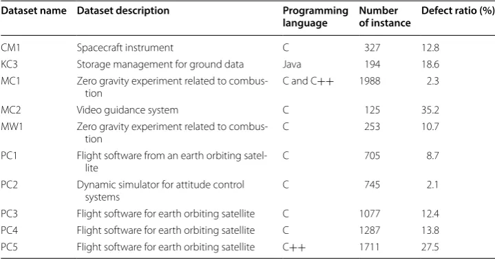
This experiment uses ten of the NASA Metrics Data Program (MDP) public dataset repositories that have been commonly used to study the software defect prediction. Table 1 summarizes those datasets. Each dataset consists of hundreds to thousands of program module entities [36, 37] with different numbers in the defect proportions. The original NASA MDP dataset repositories may need to be cleaned to remove the data redundancy and inconsistency to get more feasible for analyzing purposes [3, 38]. All

Table 1 NASA MDP datasets

Dataset name Dataset description Programming

language Number of instance Defect ratio (%)

CM1 Spacecraft instrument C 327 12.8 KC3 Storage management for ground data Java 194 18.6 MC1 Zero gravity experiment related to

combus-tion C and C++ 1988 2.3 MC2 Video guidance system C 125 35.2 MW1 Zero gravity experiment related to

combus-tion C 253 10.7

PC1 Flight software from an earth orbiting

satel-lite C 705 8.7

PC2 Dynamic simulator for attitude control

public datasets in this study are online available, which are provided by Klainfo [39] and Shepperd et al. [40].

Data preprocessing

As shown in Algorithm 1 and Algorithm 2, the preprocessing step using z-score trans-formation is added in both algorithms. The transtrans-formation aims to standardize the met-ric values so that all metmet-rics have the same value scale on the model development. The z-score transformation is formulated in Eq. 14.

where yi is the metric vector of i, ¯yi is the mean of yi , si is the standard deviation of yi , and y´i is the normalized value of yi.

Experiment design

Both of the proposed and baseline methods in this study have two main processes that are clustering and labeling, as shown in Algorithm 1 and Algorithm 2. Before carrying out those main processes, the data preprocessing is performed to improve the dataset quality for analysis purpose. In this preprocessing, the dataset is standardized by the z-score transformation in Eq. 14 to improve the data normalization and features scaling. The main experiments are then sequentially taken as follows.

• Clustering: The clustering process is partitioning process to generate the defect and clean clusters. The clustering performance is evaluated using Davies Bouldin Index (DBI) that is computed using Eq. 15. The DBI is a universal measure that is usually used to validate any clustering performance as the internal validation.

• Labeling: The labeling process is classification process to obtain the predicted class of all entities in each cluster using the row sum criterion in Eq. 12. The labeling perfor-mance is evaluated using some measures, such as precision, recall, accuracy, AUC, and error rates that are computed using Eqs. 17–21, respectively.

The study is conducted using Matlab software to evaluate both Algorithm 1 and Algo-rithm 2 with the prepared datasets.

Performance evaluations

For clustering performance, the clustering algorithm is evaluated using an internal vali-dation that is measured by the DBI, as follows:

where k is the number of all clusters, and DB_ij is calculated as follows:

(14) ´

yi= yi− ¯yi

si ,

(15) DBI= 1

k

k

i=1

max

j�=i DBij,

(16)

DB_ij= σµi+σµj

where µi is the cluster mean of Ci , µj is the mean of cluster Cj , δ(µi,µj) is the distance between cluster mean of µi and µj , while σµi and σµj are the standard deviation of clus-ter Ci and Cj , respectively. The smaller DBI indicates the better clustering, which means the predicted clusters are well partitioned because of the distance between each cluster means is large [20, 33, 36].

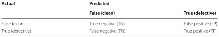
For labeling performance, the predicted labels are compared to the actual labels using confusion matrix for labeling performance evaluation [41]. The confusion matrix presents the number of predicted labels in columns and the number of actual labels in rows [16, 33], as shown in Table 2, which is constructed by these following elements:

• True negative (TN): The number of clean entities that the classifier predicts as clean. • False positive (FP): The number of clean entities that classifier predicts as defective. • False negative (FN): The number of defective entities that classifier predicts as clean. • True positive (TP): The number of defective entities that the classifier predicts as

defective.

The prediction performance measurements [33, 41–43] are then computed using the confusion matrix elements, as follows:

• Precision (PRE), which is measured by the fraction of true positive with all predicted defective entities.

• Recall (REC), which is measured by the fraction of true positive with all actual defec-tive entities. This metric is also called as true posidefec-tive rate (TPR).

• Accuracy (ACC), which is measured by the fraction of all correct predicted entities with all total entities.

• Area under curve (AUC), which is measured by the area under curve of ROC (the receiver operating characteristics). The ROC itself is constructed by the curves of true positive rate across false positive rate. The true positive rate (TPR) and false pos-itive rate (FPR) are computed using Eqs. 18 and 20, respectively [20].

(17)

PRE= TP TP+FP

(18) REC= TP

TP+FN

(19) ACC= TP+TN

TP+FP+FN+TN Table 2 Confusion matrix

Actual Predicted

False (clean) True (defective)

• Error rates (ERR) or misclassified error, which is measured by the fraction all incor-rect predicted entities with all total entities.

Validation method

Validation method is performed by comparing the proposed method performances to the baseline method. The significance of performance differences between the proposed and baseline methods are validated using the Wilcoxon signed-rank test [44, 45] at the 95% level of confidence. The Wilcoxon signed-rank is a nonparametric statistical test. Thus it does not need any assumptions about the dataset distribution. The validation test uses the null hypothesis H0 based on the median difference between pairs of data samples. This hypothesis is then tested using the p value for a decision making whether the null hypothesis is accepted or rejected [36, 46]. The p value is a probability associated with the critical value that a Type I error (false positive) is allowed. These are the follow-ing hypotheses for this study.

• H0(1) : There is no difference in cluster compactness between the proposed and base-line methods.

• H0(2) : There is no difference in precision performance between the proposed and baseline methods.

• H0(3) : There is no difference in recall performance between the proposed and

base-line methods.

• H0(4) : There is no difference in accuracy performance between the proposed and baseline methods.

• H0(5) : There is no difference in error rates between the proposed and baseline

meth-ods.

• H0(6) : There is no difference in AUC performance between the proposed and base-line methods.

All of the null hypotheses will be tested separately using the two-tailed Wilcoxon signed-rank test at the 95% level of confidence (i.e., p<0.05). If the p value is less than 0.05, then the null hypothesis is rejected, and the performances of both methods are significantly different. Otherwise, the null hypothesis is accepted.

Results and discussion

This experiment is conducted to evaluate the performances of the proposed method and comparing those performances to the baseline. The proposed and baseline methods are summarized in Algorithm 1 and Algorithm 2, respectively. As explained in " Experimen-tal setup" section, both the proposed and baseline methods are performed on the signed Laplacian matrix, which is constructed by Eq. 6.

(20)

FPR= FP

FP+TN

(21) ERR= FP+FN

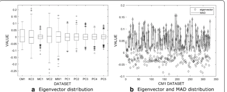
The data preprocessing, which follows step 1 in Algorithm 1 and Algorithm 2, is per-formed to standardize the dataset on the same scale. The clustering process of both the proposed and baseline algorithm follows step 2 to step 7 in Algorithm 1 and step 2 to step 6 in Algorithm 2. Step 2 and step 3 are constructing the adjacency matrix and the absolute of adjacency matrix using Eqs. 5 and 6, respectively. Step 4 is constructing the signed Laplacian matrix in Eq. 9 from the absolute of adjacency matrix in step 3. The signed Laplacian matrix is then decomposed to get the eigenvalues and eigenvectors using Eq. 10 correspond to the step 5. Figure 1a shows the eigenvectors distribution for all datasets. Almost all of the eigenvectors come with outliers in their distribution. If the zero value threshold is used to generate clusters on those eigenvectors, it may produce clusters with low compactness in cluster memberships.

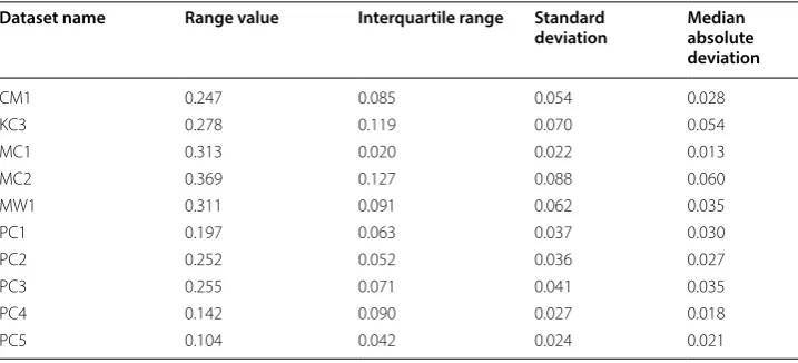
In this study, the proposed method considers the eigenvector’s values dispersion meas-ure using the MAD value to determine the new threshold. The MAD value is computed using Eq. 1. Figure 1b illustrates the comparison example between the eigenvector dis-persion and its MAD on CM1 dataset. It shows that the MAD value overcomes the out-liers in the eigenvector dispersion. The MAD value represents the eigenvector values position and does not reflect the changes of the eigenvector values. Table 3 presents the dispersion measures of eigenvectors for all datasets, such as range, interquartile range, standard deviation, and MAD.

The next step is the partitioning process to generate defective and clean clusters. The second smallest eigenvalue of the Laplacian matrix is chosen to define the selected eigenvector for the partitioning process. Besides, the partitioning process also needs a partitioning threshold. The proposed method uses the median absolute deviation of the selected eigenvector, while the baseline method used the zero value as the partition thresholds. The MAD value of the selected eigenvector is computed using Eq. 1, corre-sponds the step 6 in Algorithm 1. Both of these thresholds are then used to generate the clusters, corresponds the step 7 in Algorithm 1 and step 6 in Algorithm 2, respectively. The cluster memberships of both proposed and baseline methods follow Eqs. 11 and 13, respectively.

In the proposed method, the defective cluster is constructed to group all entities which its eigenvalue greater than the MAD threshold—otherwise, the clean cluster is

Table 3 Eigenvector dispersion measures

Dataset name Range value Interquartile range Standard

deviation Median absolute deviation

constructed to group all entities which its eigenvector less or equals than the MAD threshold. In the baseline method, the defective cluster is constructed to group all enti-ties which its eigenvalue greater than zero—otherwise, the clean cluster is constructed to group all entities which its eigenvector less or equals than zero. Table 4 shows the dis-tribution of cluster memberships using both proposed and baseline methods.

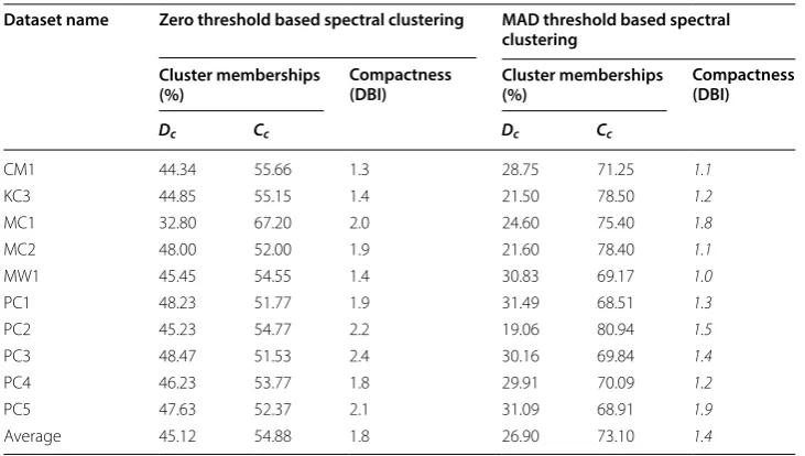
The proposed method detects 26.90% of all entities as defective (i.e., in the defec-tive cluster) and 73.10% of all entities as clean (i.e., in the defecdefec-tive cluster). Whereas, the baseline method detects 45.12% of all entities as defective and 54.88% of all entities as clean. Based on these results and compared to the number of defective in Table 1, the proposed method can produce clusters with better cluster memberships than the Table 4 Clusters membership and performance

Dc is the predicted defective cluster; Cc is the predicted clean cluster

The italicized values indicate the better performance

Dataset name Zero threshold based spectral clustering MAD threshold based spectral clustering

Cluster memberships

(%) Compactness (DBI) Cluster memberships (%) Compactness (DBI)

Dc Cc Dc Cc

CM1 44.34 55.66 1.3 28.75 71.25 1.1

KC3 44.85 55.15 1.4 21.50 78.50 1.2

MC1 32.80 67.20 2.0 24.60 75.40 1.8

MC2 48.00 52.00 1.9 21.60 78.40 1.1

MW1 45.45 54.55 1.4 30.83 69.17 1.0

PC1 48.23 51.77 1.9 31.49 68.51 1.3

PC2 45.23 54.77 2.2 19.06 80.94 1.5

PC3 48.47 51.53 2.4 30.16 69.84 1.4

PC4 46.23 53.77 1.8 29.91 70.09 1.2

PC5 47.63 52.37 2.1 31.09 68.91 1.9

Average 45.12 54.88 1.8 26.90 73.10 1.4

baseline. The proposed method groups the entities based on their eigenvector positions that are measured by its distance to the median. Whereas, the zero threshold groups the entities based on their eigenvector difference values with the zero. Figure 2 shows the example of the cluster memberships on CM1 dataset that are produced by both the pro-posed and baseline methods.

The clustering performances of both methods are evaluated using the cluster com-pactness, which is measured by the DBI in Eq. 15. Table 4 shows the DBI values, where the proposed method outperforms the baseline for all datasets. The cluster compact-ness averages of both the proposed and baseline methods are 1.4 DBI and 1.8 DBI, respectively. This achievement corresponds with the increase in the number of cluster membership as referred on Table 4. The clustering performance difference between the proposed and baseline methods is validated using the two-tailed Wilcoxon signed-rank test at 95% level of confidence. The observed p value of this test is 0.001. Hence, the null hypothesis H0(1) is rejected. This significance test concludes that the proposed method can produce better cluster compactness than the baseline method.

Following Algorithm 1 and Algorithm 2, the last step is labeling all cluster members as defective or clean classes. The label of each entity is obtained using the heuristic row sum criterion in Eq. 12 by comparing the row sum of the entity with the average row sum of its cluster. The classifier performances are then evaluated using precision, recall, accuracy, AUC, and also error rates, which are computed using Eq. 17–21, respectively. Table 5 shows all of these performances using both the proposed and baseline methods.

In precision performance, Table 5 shows that the proposed method can improve the precision of the baseline. The precisions averages of both methods are 0.84 and 0.74, respectively. While Fig. 3a illustrates the precision performance comparison between the proposed and baseline methods for all datasets. The precision performance differ-ence has been validated using the two-tailed Wilcoxon signed-rank test at the 95% level of confidence. The observed p value is 0.005 and the null hypothesis H0(2) is rejected. Hence, the precisions of both methods are significantly different. Table 5 also shows that the proposed method outperforms the baseline in the CM1, MC1, MW1, PC1, Table 5 Performance comparison between  zero and  MAD threshold based spectral classifiers

The italicized values indicate the better performance

Dataset name Zero threshold based spectral classifier MAD threshold based spectral classifier

PRE REC ACC AUC ERR PRE REC ACC AUC ERR

CM1 0.72 0.92 0.71 0.68 0.29 0.81 0.71 0.76 0.76 0.24

KC3 0.78 0.88 0.75 0.75 0.25 0.72 0.61 0.71 0.80 0.29 MC1 0.76 0.94 0.78 0.67 0.22 0.98 0.94 0.94 0.74 0.06

MC2 0.74 0.71 0.68 0.75 0.32 0.60 0.57 0.67 0.82 0.33 MW1 0.69 0.95 0.69 0.70 0.31 0.84 0.58 0.71 0.74 0.29

PC1 0.73 0.94 0.75 0.78 0.25 0.83 0.64 0.80 0.77 0.20

PC2 0.72 0.89 0.77 0.76 0.23 0.97 0.63 0.84 0.74 0.16

PC3 0.72 0.92 0.79 0.77 0.21 0.85 0.86 0.80 0.77 0.20

PC4 0.79 0.90 0.72 0.67 0.28 0.87 0.80 0.73 0.77 0.27

PC5 0.78 0.81 0.78 0.74 0.22 0.88 0.87 0.94 0.74 0.06

PC2, PC3, PC4, and PC5 datasets. However, the proposed method underperformed in the KC3 and MC2 datasets. Related to the eigenvector’s values dispersion measure in Table 3, the KC3 and MC2 datasets have higher dispersion measures than the other datasets, especially in the interquartile range, standard deviation, and MAD values. Sta-tistically, those eigenvector’s dispersion measures affect the entities distribution. For example, the interquartile range represents the range of the middle half of the eigenvec-tor’s values distribution. The higher interquartile range indicates that the eigenveceigenvec-tor’s values spread out from the central tendency point (e.g., median). Hence, the number of both defective and clean entities in the middle-half of the eigenvector’s values distribu-tion becomes increasing. Consequently, the precision of the proposed method becomes decreasing in the KC3 and MC2 datasets and underperformed the baseline method.

In contrary to precision, the proposed method underperformed the baseline in the recall performance. As shown in Table 5, the recall values of the proposed method are smaller than the recall values of the baseline method. The recall averages of both meth-ods are 0.72 and 0.89, respectively. Figure 3b illustrates the recall performance compari-son between the proposed and baseline methods for all datasets. The recall performance difference is proven significant by the two-tailed Wilcoxon signed-rank test at the 95% level of confidence. The observed p value is 0.01 and the null hypothesis H0(3) is rejected. Hence, the recall performance of the proposed method is significantly different from the baseline method. Table 5 also shows that recall of the proposed method outperforms the baseline only in the PC5 dataset. Related to the eigenvector’s values dispersion of this dataset in Table 3, the PC5 dataset has the lowest range of eigenvector values than the other datasets. It means that the difference value between the maximum and mini-mum of the eigenvectors in the PC5 dataset is too small. Hence, almost entities spread

around the central tendency point, including both the defective and clean entities. Con-sequently, the ratio of the correct predicted defective to all the actual defective entities (i.e., recall) in the PC5 dataset becomes increasing.

Based on the precision and recall, there is a trade-off performance between the pro-posed and baseline methods. The propro-posed method has high in precision but low in the recall, while the baseline method has low in precision but high in the recall. This trade-off indicates that the proposed method can predict more precisely the actual defective, although in the small number. Whereas the baseline method can predict more defective entities, but not all of the predicted defectives are actual defectives.

In terms of accuracy, Table 5 shows that the proposed method outperforms the base-line in almost all of datasets, but underperformed in the KC3 and MC2 datasets. These lower accuracies in those two datasets might be caused by the high dispersion measures in the interquartile range, standard deviation, and MAD, as shown in Table 3. Overall, the accuracy averages of both the proposed and baseline methods are 0.79 and 0.74, respectively. Hence, the error rate of both the proposed and baseline methods are 0.21 and 0.26, respectively. It means that 79% of all entities are classified correctly using the proposed method with the misclassified rates of 21%, while the baseline method can classify 74% of all entities correctly with the misclassified rates of 26%. Those accura-cies and error rates indicate that the proposed method can predict the defective enti-ties more accurate than the baseline. The performance comparison of accuracy and error rates between the proposed and baseline methods for all datasets are illustrated in Fig. 3c, d, respectively. The accuracy performance and error rates differences are proven significant by the Wilcoxon test at the 95% level of confidence. The observed p value of accuracy performance test is 0.03, and the null hypothesis H0(4) is rejected. While the error rates difference test gives observed p value of this test is 0.04, and the null hypoth-esis H0(5) is rejected.

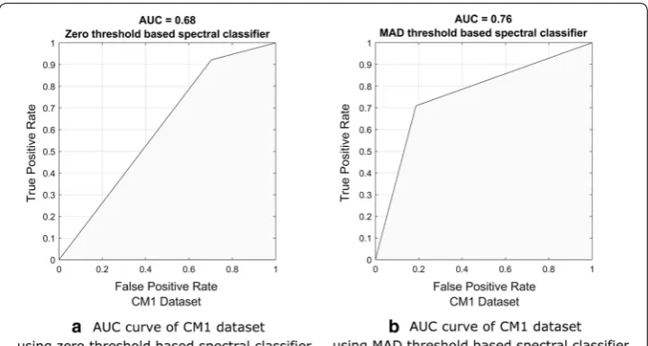
In terms of AUC, Table 5 shows that the proposed method outperforms the baseline in almost all of datasets. The AUC averages of both methods are 0.77 and 0.73, respectively. It means that the abilities to distinguish the defective and clean classes of both methods are 77% and 73%, respectively. The AUC performance difference is proven significant by the two-tailed Wilcoxon signed-rank test at the 95% level of confidence. The observed p value of this test is 0.01, and the null hypothesis H0(6) is rejected. Figure 4 illustrates the example of the AUC curve for the CM1 dataset. The AUC itself is the area under the ROC that is constructed using the true positive rate (TPR) across the false positive rate (FPR), which are computed by Eqs. 18 and 20, respectively.

Conclusion

The median absolute deviation threshold has been presented in this paper to address the zero threshold issues in the spectral classifier based unsupervised software defect prediction. The median absolute deviation, as a dispersion measure, is proposed as the partitioning threshold to reduce the predominantly cluster issue when the eigenvec-tor values of spectral graph matrix are mostly positives. The median absolute deviation threshold is also designed to address the eigenvector values outliers issue. Thus, the objective of this study is generally to improve the performances of zero value threshold based spectral classifier in unsupervised software defect prediction through the median absolute deviation threshold based spectral classifier.

Experimental results show that the proposed method can improve both clustering and classification. The proposed method produces better cluster memberships and increase cluster compactness. Which means there is an improvement in the numbers of entities that are separated correctly into the predicted clusters. This resulting clusters affect the classification performance improvement. The accuracy and misclassified rates of the median absolute deviation threshold based spectral classifier outperformed the zero threshold value based spectral classifier. In the AUC performance, the median absolute deviation threshold based spectral classifier also performs better in the ability to dis-tinguish the defective and clean classes. In the precision and recall performances, the median absolute deviation threshold based spectral classifier high in precision although low in the recall. Based on those achievements, this study concludes that the median absolute deviation threshold based spectral classifier not only able to overcome the zero value threshold issues in the spectral classifier. But, it can also improve the zero value threshold based spectral classifier performances. The median absolute deviation threshold based spectral classifier method is an unsupervised approach with no need of training dataset. Thus, there is a significant potential to generalize the proposed method on the new software projects or an established software project with lacks in training dataset.

Abbreviations

MAD: median absolute deviation; MDP: metrics data program; DBI: Davies Bouldin index; DB: Davies Bouldin; TP: true positive; TN: true negative; FP: false positive; FN: false negative; PRE: precision; REC: recall; TPR: true positive rates; FPR: false positive rates; ACC : accuracy; ERR: error rates; AUC : area under curve; ROC: receiver operating characteristics. Acknowledgements

Not applicable. Authors’ contributions

All authors contributed both the concepts and contents of this study. AM provided the manuscript under supervised by TBA and RF. All authors also performed discussion intensively for contents improvement. All authors read and approved the final manuscript.

Funding Not applicable. Availability of datasets

The datasets used in this paper are publicly online available as described in "Dataset preparation" section. Competing interests

The authors declare that they have no competing interests. Author details

1 _{Department of Electrical and Information Engineering, Faculty of Engineering, Universitas Gadjah Mada, Jl. Grafika No.} 2, Kampus UGM, Yogyakarta 55281, Indonesia. 2 _{Department of Informatics Engineering, Faculty of Computer Science,} Universitas Dian Nuswantoro, Jl. Imam Bonjol No. 207, Semarang 50131, Jawa Tengah, Indonesia.

Received: 18 July 2019 Accepted: 9 September 2019

References

1. Punitha K, Chitra S. Software defect prediction using software metrics: a survey. In: Proceedings of the 2013 inter-national conference on information communication and embedded systems (ICICES); 2013. p. 555–8. https ://doi. org/10.1109/ICICE S.2013.65083 69.

2. Petersen K. Measuring and predicting software productivity: a systematic map and review. Inf Softw Technol. 2011;53(4):317–43. https ://doi.org/10.1016/j.infso f.2010.12.001.

3. Zhang F, Zheng Q, Zou Y, Hassan AE. Cross-project defect prediction using a connectivity-based unsupervised classi-fier. In: Proceedings of the 38th international conference on software engineering ICSE; 2016. p. 309–20. https ://doi. org/10.1145/28847 81.28848 39.

4. Nam J, Fu W, Kim S, Menzies T, Tan L. Heterogeneous defect prediction. IEEE Trans Softw Eng. 2018;44(09):874–96. https ://doi.org/10.1109/TSE.2017.27206 03.

5. Singh P, Verma S, Vyas OP. Software fault prediction at design phase. J Electr Eng Technol. 2015;9(5):1739–45. https :// doi.org/10.5370/JEET.2014.9.4.742.

6. Ryu D, Baik J. Effective multi-objective Naive Bayes learning for cross-project defect prediction. Appl Soft Comput. 2016;49:1062–77. https ://doi.org/10.1016/j.asoc.2016.04.009.

7. Cheng M, Wu G, Jiang M, Wan H, You G, Yuan M. Heterogeneous defect prediction via exploiting correlation sub-space. In: Proceedings of the 28th international conference on software engineering and knowledge engineering SEKE 2016; 2016. p. 171–6. https ://doi.org/10.18293 /seke2 016-090.

8. Yeh Y, Huang C, Wang YF. Heterogeneous domain adaptation and classification by exploiting the correlation sub-space. IEEE Trans Image Process. 2014;23(5):2009–18. https ://doi.org/10.1109/TIP.2014.23109 92.

9. Fu W, Menzies T. Revisiting unsupervised learning for defect prediction. In: Proceedings of the 2017 11th joint meet-ing on foundations of software engineermeet-ing ESEC/FSE 2017; 2017. p. 72-83. https ://doi.org/10.1145/31062 37.31062 57.

10. Yang J, Qian H. Defect prediction on unlabeled datasets by using unsupervised clustering. In: Proceedings the 2016 IEEE 18th international conference on high performance computing and communications; IEEE 14th international conference on Smart City; IEEE 2nd international conference on data science and systems (HPCC/SmartCity/DSS); 2016. p. 465–72. https ://doi.org/10.1109/HPCC-Smart City-DSS.2016.0073.

11. Wahono RS. A systematic literature review of software defect prediction: research trends, datasets, methods and frameworks. J Softw Eng. 2015;1(1):1–16. https ://doi.org/10.1049/iet-sen.2011.0132.

12. Azam NF, Viktor HL. Spectral clustering: an explorative study of proximity measures. In: Fred A, Dietz JLG, Liu K, Filipe J, editors. Knowledge discovery, knowledge engineering and knowledge management. IC3K 2011. Communica-tions in computer and information science, vol. 348. Berlin: Springer; 2013. https ://doi.org/10.1007/978-3-642-37186 -8_4.

13. Marjuni A, Adji TB, Ferdiana R. Unsupervised software defect prediction using signed Laplacian-based spectral classi-fier. Soft Comput. 2019;2019:1–12. https ://doi.org/10.1007/s0050 0-019-03907 -6.

14. Zhong S, Khoshgoftaar TM, Seliya N. Unsupervised learning for expert-based software quality estimation. In: Pro-ceedings of the eighth IEEE international conference on high assurance systems engineering HASE 2004; 2004. p. 149–55. https ://doi.org/10.1109/HASE.2004.12817 39.

16. Bishnu PS, Bhattacherjee V. Software fault prediction using quad tree-based k-means clustering algorithm. IEEE Trans Knowl Data Eng. 2012;24(6):1146–50. https ://doi.org/10.1109/TKDE.2011.163.

17. Abaei G, Rezaei Z, Selamat A. Fault prediction by utilizing self-organizing map and threshold. In: Proceedings of the international conference on control system, computing and engineering, ICCSCE 2013; 2013. p. 465–70. https ://doi. org/10.1109/ICCSC E.2013.67200 10.

18. Nam J, Kim S. CLAMI: defect prediction on unlabeled datasets. In: Proceedings of the 30th IEEE/ACM international conference on automated software engineering ASE 2015; 2015. p. 452–63. https ://doi.org/10.1109/ASE.2015.56. 19. Shi J, Malik J. Normalized cuts and image segmentation. IEEE Trans Pattern Anal Mach Intell. 2000;22(8):888–905.

https ://doi.org/10.1109/34.86868 8.

20. Aggarwal C, Reddy CK. Data clustering: algorithms and applications. Boca Raton: CRC Press, Taylor and Francis Group; 2014.

21. Wang X, Davidson I. Active spectral clustering. In: Proceedings of the 10th IEEE international conference on data mining; 2010. p. 561–8. https ://doi.org/10.1109/ICDM.2010.119.

22. Wacquet G, Caillault EP, Hamad D, Hébert PA. Constrained spectral embedding for K-way data clustering. Pattern Recogn Lett. 2013;4(9):1009–17. https ://doi.org/10.1016/j.patre c.2013.02.003.

23. Kunegis J, Schmidt S, Lommatzsch A, Lerner J, De Luca EW, Albayrak S. Spectral analysis of signed graphs for cluster-ing, prediction and visualization. In: Proceedings of the SIAM international conference on data mining SDM 2010; 2010. p. 559–70. https ://doi.org/10.1137/1.97816 11972 801.49.

24. Dodge Y. Mean absolute deviation. The concise encyclopedia of statistics. New York: Springer; 2008. p. 348. 25. Mantaj A, Pater R, Wagner W. Aspects of linear and median correlation coefficients matrix. Folia Oecon.

2010;2010(235):307–27.

26. Stephanie. Median absolute deviation. 2014. https ://www.stati stics howto .datas cienc ecent ral.com/media n-absol ute-devia tion/.

27. Median absolute deviation. In: Encyclopedia of statistics in behavioral science. https ://doi.org/10.1002/04700 13192 .bsa38 4.

28. Rousseeuw PJ, Croux C. Alternatives to the median absolute deviation. J Am Stat Assoc. 1993;88(424):1273–83. https ://doi.org/10.1080/01621 459.1993.10476 408.

29. Pham-Gia T, Hung TL. The mean and median absolute deviations. Math Comput Model. 2001;34(7):921–36. https :// doi.org/10.1016/S0895 -7177(01)00109 -1.

30. Arce GR, Li Y. Median power and median correlation theory. IEEE Trans Signal Process. 2002;50(11):2768–76. https :// doi.org/10.1109/TSP.2002.80409 2.

31. Ahad NA, Abdullah S, Zakaria NA, Yahaya SSS, Yusof N. Median based robust correlation coefficient. In: AIP Confer-ence Proceedings. 2017;1905(1):050002:1–050002:5. https ://doi.org/10.1063/1.50122 21.

32. Hogel J, Schmid W, Gaus W. Robustness of the standard deviation and other measures of dispersion. Biom J. 1994;36(4):411–27. https ://doi.org/10.1002/bimj.47103 60403 .

33. Zaki MJ, Wagner M. Data mining and analysis. New York: Cambridge Univerity Press; 2014.

34. Malgorzata L, Slawomir TW. Clustering based on eigenvectors of the adjacency matrix. Int J App Math Comput Sci. 2018;28(4):771–86. https ://doi.org/10.2478/amcs-2018-0059.

35. Knyazev AV. Signed Laplacian for spectral clustering revisited. ArXiv, abs/1701.01394. arxiv :pdf/1701.01394 .pdf. 2017. 36. Tomar D, Agarwal S. Prediction of defective software modules using class imbalance learning. Appl Comput Intell

Soft Comput. 2016;2016:1–12. https ://doi.org/10.1155/2016/76582 07.

37. Gray D, Bowes D, Davey N, Sun Y, Christianson B. Reflections on the NASA MDP data sets. IET Softw. 2012;6(6):549– 58. https ://doi.org/10.1049/iet-sen.2011.0132.

38. Shepperd M, Song Q, Sun Z, Mair C. Data quality: some comments on the NASA software defect datasets. IEEE Trans Softw Eng. 2013;39(9):1208–15. https ://doi.org/10.1109/TSE.2013.11.

39. Klainfo NASA MDP software defect dataset. 2016. https ://githu b.com/klain fo/NASAD efect Datas et.

40. Shepperd M, Song Q, Sun Z, Mair C. NASA MDP software defects datasets. 2018. https ://figsh are.com/colle ction s/ NASA_MDP_Softw are_Defec ts_Data_Sets/40549 40.

41. Hall T, Beecham S, Bowes D, Gray D, Counsell S. A systematic literature review on fault prediction performance in software engineering. IEEE Trans Softw Eng. 2012;38(6):1276–304. https ://doi.org/10.1109/TSE.2011.103. 42. Davies ER. Machine learning: probabilistic methods. In: Computer vsion. 5th ed. Cambridge: Academic Press; 2018.

p. 399–451.

43. MLWiki Evaluation of binary classifiers. 2015. http://mlwik i.org/index .php/Evalu ation _of_Binar y_Class ifier s. 44. Rey D, Neuhauser M. Wilcoxon signed-rank test. In: Lovric M, editor. International encyclopedia of statistical science.

Heidelberg: Springer; 2011.

45. Ren J, Qin K, Ma Y, Luo G. On software defect prediction using machine learning. J Appl Math. 2014;2014:1–9. https ://doi.org/10.1155/2014/78543 5.

46. Ryu D, Choi O, Baik J. Value-cognitive boosting with a support vector machine for cross-project defect prediction. Empir Softw Eng. 2016;21(1):43–71. https ://doi.org/10.1007/s1066 4-014-9346-4.

Publisher’s Note