Vol. 5 Issue 8, August - 2019
Optimization Of Resources in a PYME Of the
Textil Sector: An Lineal Programming Approach
Ing. Jorge Manuel Barrios Sanchez
Master Degree Student Department of Multidisciplinary Sede Yuriria, Universidad de Guanajuato
Yuriria Mexico [email protected]
Dr. Roberto Baeza Serrato
Research Profesor
Department of Multidisciplinary Sede Yuriria, Universidad de Guanajuato
Yuriria-Mexico [email protected]
Abstract—A linear programming model is
presented as a tool to maximize profits in a SME located in the south of Guanajuato. An Excel spreadsheet was designed and developed to solve the model, using the revised simplex model. Time, inputs and demand constrictions were integrated for the seven main products. Ten iterations of the revised simplex method were made to obtain the model optimization; the right sequence of processes results in a $11,830 MXN daily gain. This model can be replicated in any textile SME and be a prototype for any productive enterprise.
Keywords—lineal programming; optimization ; revised simplex method.
The textile sector is considered one of the most developed activities, nevertheless it shows a high capacity of innovation and new development, like the ones needed for season changes, functional and aesthetical modifications required by the cultural evolution, and specially the pressure of demanding customers, and the arrival of new competitors; that’s the reason innovation is a continuous process, making it a stable course in the sector and a strategic point for the SMEs [1]. In México, the SMEs are the 42% of the country enterprises, contributing to 31.5% of the employment and almost 37.0% of the Gross Domestic Product(GDP), also it is the backbone of the national economy, the reason being the trade agreements of the last years [2].
Decision making in this sector is a difficult task in which the efficient use of inputs, time and money is crucial. Linear programming models are a powerful tool to reach the optimization objectives. Many problems of operation research can be solved as linear programming applications. Special cases as the flux in a network or the movement of merchandises are so important that the research in those areas has produced many algorithms to solve them [3].
Today, optimization is a normal procedure in sciences, engineering and business [4]. The revised simplex method requires less calculation than other methods. Basically, it performs calculations only in the vector of the non-basic variables and registers in memory all the information of the basic ones [5].
In the city of Moroleón, located at the south of Guanajuato, lies a great quantity of SMEs that specialize in the knitting process. These have become
the main center of textile production and commercialization in the region.
The case study is focused in a textile enterprise called NAVY SEAL S. DE R.L. DE C.V. in the city of Moroleón, that produces clothes and knitted outerwear. The objective is to optimize the resources of the enterprise, having as a reference the time needed for each process, the inputs and the minimal sales needed to continue its operation.
I. LITERATURE REVIEW
In this section the results of an exhaustive investigation for previous works involved in operation research with the revised simplex model are presented.
time frame in the normal operation of the lot, using a revised simplex model.
The applications cited show applications of the simplex and simplex method revised, in various productive and service sectors. There is a shortage of developments of linear programming models in SMEs, due to the tacit knowledge they have, reason for the present research to present an application of a linear programming model that what contributes to the review of literature for small and medium enterprises in the textile sector.
II. METHODOLOGY
In this section, the methodology designed for performing the research is presented. See Table 1.
TABLE I. RESEARCH METHODOLOGY.
PHASE AIM PROCEDURE
Case study Identification.
Identify the processes, costs and sales of every one of the products of the case study for a better knowledge of every one of these products.
Through a visit to the firm and by
studying the
products offered by the textile company.
Theoretical Base
Examine the state of the art from applications of the revised simplex method in order to have a guide on how it has been implemented. Through databases, scientific articles. Decide decision variables
Identify the decision variables to know the elements on which to decide.
Through a
selection of the
best selling
garments in the company.
Decide objetive function
Establish the objective function to express what is intended to maximize
The utility of each of the decision
variables is
determined
Decide Restrictions
Define the restrictions of resources,
production and demand to denote the limitations that are available.
Through an
interview with the
head of
production, the restrictions that are had.
Results and conclusions.
Application of the revised simplex method to obtain maximum utility when optimizing resources and time.
Excel Template.
A. Case study identificaction
To perform this research, the PYME NAVY SEAL S. DE R.L DE C.V was selected as case study. The company has different processes for the making of each of the garments produced by the company; 1- Weaving process that is performed by a circular textile machine 2- Cutting process 3- confection 4- finished of the garment and finally the packaging for shipment to the products manufactured by the company, were selected which are the most manufactured and sold by the company. See table 2.
TABLE II. BESTSELLING PRODUCTS OF THE COMPANY TEXTILES NAVY SEAL S. DE R.L DE C.V
Product Sale price Sale cost
Tank top 25 17
Short sleeve
blouse 35 25
Large sleeve
blouse 60 44
Basic boxer 37 28
Fajilla 36 22
Scarlett blouse 46 33
Boxer designs 55 39
B. Time restriction
The production manager assisted in the data acquisition of the times of each one of the products. The standardized times in the processes of each of the aforementioned products can be seen in Table 3.
Table III. TIME RESTRICTION.
Minutes
Product Knitting Cutting Making Finished
Tank Top 04:00 00:00 01:00 00:30 Short
Sleeve Blouse
06:30 01:12 02:00 01:00
Large Sleeve Blouse
12:00 01:30 02:30 01:30
Basic
Boxer 04:30 00:18 01:30 01:00 Fajilla 06:30 00:00 03:30 01:30 Scarlett
Blouse 05:30 00:00 04:00 02:00 Boxer
Designs 05:30 00:09 01:30 01:00 Time
Restriction 96 hours
28:30
hours 80 hours 80 hours
Vol. 5 Issue 8, August - 2019 C. Resourses restriction
The amount of thread required for each of the garments can be seen in table 4.
Table IV. TIME RESTRICTION.
Product Thread Quantity (Kg)
Tank top 0.07
Short sleeve blouse 0.11
Large sleeve blouse 0.16
Basic boxer 0.1
Fajilla 0.13
Scarlett blouse 0.1
Boxer designs 0.11
There is a daily amount of 125 kg of thread for the realization of the garments. The amount of thread is mainly used in the weaving process.
D. Production restriction.
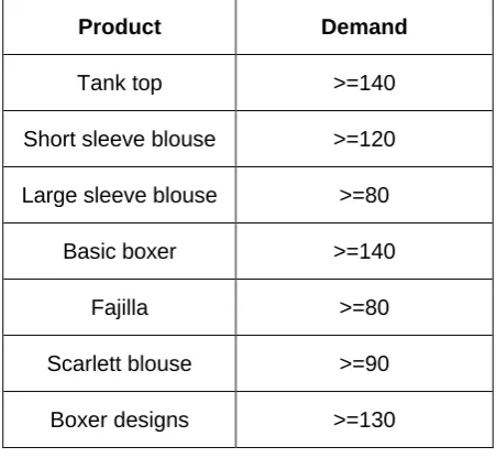
To produce the seven products, there is a minimum production of each of these garments that are sold daily to different customers that the company has, mainly to Coppel company. The minimum sales that each of the products must have are shown in table 5.
TABLE V. MINIMAL GARMENT PRODUCTION
Product Demand
Tank top >=140
Short sleeve blouse >=120
Large sleeve blouse >=80
Basic boxer >=140
Fajilla >=80
Scarlett blouse >=90
Boxer designs >=130
III. RESULTS.
Mathematical models in linear programming have three basic components that are: Decision variables, objective function and constraints. The decision variables are defined, which represent the elements on which they must be decided.
X1= # of tank top to produce
X2=# of short sleeve blouse to produce
X3=# of large sleeve blouse to produce
X4=# of basic boxer to produce
X5=# of fajilla to produce
X6=# of scarlett blouse to produce
X7=# of boxer designs to produce
Function Objective:
The objective function expresses what you want to maximize. the profit from the sale of the seven main products. See Equation 1
𝑍 = 8x1 + 10x2 + 16x3 + 9x4 + 14x5 + 13x6 + 16x7 (1)
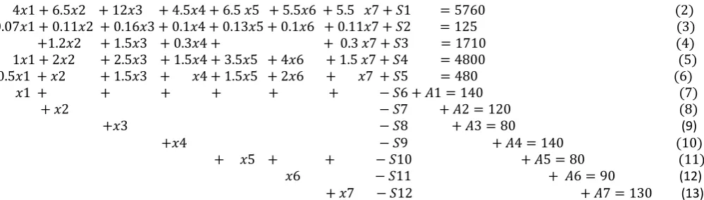
The restrictions count the resources that are available which are limited. Table VI shows the restrictions of time, material and demand.
TABLE VI. SHOWS THE TIME, MATERIAL AND DEMAND RESTRICTIONS.
X1 X2 X3 X4 X5 X6 X7 B
4 6.5 12 4.5 6.5 5.5 5.5 <=5760 0.07 0.11 0.16 0.1 0.13 0.1 0.11 <=125
0 1.2 1.5 0.3 0 0 0.3 <=1710 1 2 2.5 1.5 3.5 4 1.5 <=4800 0.5 1 1.5 1 1.5 2 1 <=4800
1 0 0 0 0 0 0 >=140
0 1 0 0 0 0 0 >=120
0 0 1 0 0 0 0 >=80
0 0 0 1 0 0 0 >=140
0 0 0 0 1 0 0 >=80
0 0 0 0 0 1 0 >=90
0 0 0 0 0 0 1 >=130
It can be analyzed that the values that are worth zero within the matrix of restrictions are processes that are not necessary in the elaboration of each of the garments.
Rows 1,3,4 and 5 are the times of the processes explained in table 3. Row 2 is the resource restriction in Kilograms and row 6 through 12 are the minimum production constraints that the company has in the seven products.
4𝑥1 + 6.5𝑥2 + 12𝑥3 + 4.5𝑥4 + 6.5 𝑥5 + 5.5𝑥6 + 5.5 𝑥7 + 𝑆1 = 5760 (2)
0.07𝑥1 + 0.11𝑥2 + 0.16𝑥3 + 0.1𝑥4 + 0.13𝑥5 + 0.1𝑥6 + 0.11𝑥7 + 𝑆2 = 125 (3)
+1.2𝑥2 + 1.5𝑥3 + 0.3𝑥4 + + 0.3 𝑥7 + 𝑆3 = 1710 (4)
1𝑥1 + 2𝑥2 + 2.5𝑥3 + 1.5𝑥4 + 3.5𝑥5 + 4𝑥6 + 1.5 𝑥7 + 𝑆4 = 4800 (5)
0.5𝑥1 + 𝑥2 + 1.5𝑥3 + 𝑥4 + 1.5𝑥5 + 2𝑥6 + 𝑥7 + 𝑆5 = 480 (6)
𝑥1 + + + + + + − 𝑆6 + 𝐴1 = 140 (7)
+ 𝑥2 − 𝑆7 + 𝐴2 = 120 (8)
+𝑥3 − 𝑆8 + 𝐴3 = 80 (9)
+𝑥4 − 𝑆9 + 𝐴4 = 140 (10)
+ 𝑥5 + + − 𝑆10 + 𝐴5 = 80 (11)
𝑥6 − 𝑆11 + 𝐴6 = 90 (12)
+ 𝑥7 − 𝑆12 + 𝐴7 = 130 (13)
The next step is to define the matrix (B) that has the identity and It will be the one that is initially in the base on the revised simplex method.
To perform the revised Simplex Method, the following operations must be followed in order.
1- Find (𝐵−1)
2- 𝑋𝑏 = 𝐵−1∗ 𝑏.
3- 𝑍𝑖𝑖 = 𝐶𝑏 ∗ 𝐵−1
4- 𝑔𝑎𝑖𝑛 = 𝐶𝑗 − 𝑍𝑗
5- 𝑍 = 𝐶𝑏 ∗ 𝑋𝑏
6- 𝑍𝑖 = 𝑍𝑖𝑖 ∗ 𝐴
7-The input variable is selected according to the highest value obtained.
8-Xb is divided by b (Xb/b) to calculate teta and the lowest value is selected as output variable.
9- The input variable is selected and replaced by the output variable and its values in the base are changed. The above steps are repeated to find the optimal pattern.
The variables found within the base can be seen in the first column of Table VII. The cost coefficients of the variables within the base are located in row CB. It can be observed the base matrix of the first iteration.
Table VII. Matrix identity base of the first iteration.
0 0 0 0 0 -16 -16 -16 -16 -16 -16 -16
Xj S1 S2 S3 S4 S5 A1 A2 A3 A4 A5 A6 A7
MATRIX B
S1 1 0 0 0 0 0 0 0 0 0 0 0
S2 0 1 0 0 0 0 0 0 0 0 0 0
S3 0 0 1 0 0 0 0 0 0 0 0 0
S4 0 0 0 1 0 0 0 0 0 0 0 0
S5 0 0 0 0 1 0 0 0 0 0 0 0
A1 0 0 0 0 0 1 0 0 0 0 0 0
A2 0 0 0 0 0 0 1 0 0 0 0 0
A3 0 0 0 0 0 0 0 1 0 0 0 0
A4 0 0 0 0 0 0 0 0 1 0 0 0
A5 0 0 0 0 0 0 0 0 0 1 0 0
A6 0 0 0 0 0 0 0 0 0 0 1 0
A7 0 0 0 0 0 0 0 0 0 0 0 1
S1 S2 S3 S4 S5 A1 A2 A3 A4 A5 A6 A7
CB 0 0 0 0 0 -16 -16 -16 -16 -16 -16 -16
ZJ 0 0 0 0 0 -16 -16 -16 -16 -16 -16 -16
Vol. 5 Issue 8, August - 2019
Table VIII shows the inverse matrix of the base, vector b of the available resource, column Xb of solution. The input variable in the first iteration is selected from the match between X3 and X7 with the most positive values, in this case with a value of 32, which are located in column four and eight, the input variable X3 is selected. The output vector with the lowest value of the Xb/Ve ratio was the artificial variable A3.
Table VIII. Inverse Matrix and first iteration results.
8 10 16 9 14 13 16 0 0 0 0 0 0 0
Xj X1 X2 X3 X4 X5 X6 X7 S6 S7 S8 S9 S10 S11 S12
INVERSE OF B b Xb Ve Teta
S1 1 0 0 0 0 0 0 0 0 0 0 0 5760 5760 12 480
S2 0 1 0 0 0 0 0 0 0 0 0 0 125 125 0.16 781.25
S3 0 0 1 0 0 0 0 0 0 0 0 0 1710 1710 1.5 1140
S4 0 0 0 1 0 0 0 0 0 0 0 0 4800 4800 2.5 1920
S5 0 0 0 0 1 0 0 0 0 0 0 0 4800 4800 1.5 3200
A1 0 0 0 0 0 1 0 0 0 0 0 0 140 140 0 ---
A2 0 0 0 0 0 0 1 0 0 0 0 0 120 120 0 ---
A3 0 0 0 0 0 0 0 1 0 0 0 0 80 80 1 80
A4 0 0 0 0 0 0 0 0 1 0 0 0 140 140 0 ---
A5 0 0 0 0 0 0 0 0 0 1 0 0 80 80 0 ---
A6 0 0 0 0 0 0 0 0 0 0 1 0 90 90 0 ---
A7 0 0 0 0 0 0 0 0 0 0 0 1 130 130 0 ---
Z -12480
Zj -16 -16 -16 -16 -16 -16 -16 16 16 16 16 16 16 0
Cj-Zj
24 26 32 25 30 29 32 -16 -16 -16 -16 -16 -16 0
In the next iteration non-negative solutions for Xb are validated. The objective function gives a solution of -12840, which will be increased in each iteration.
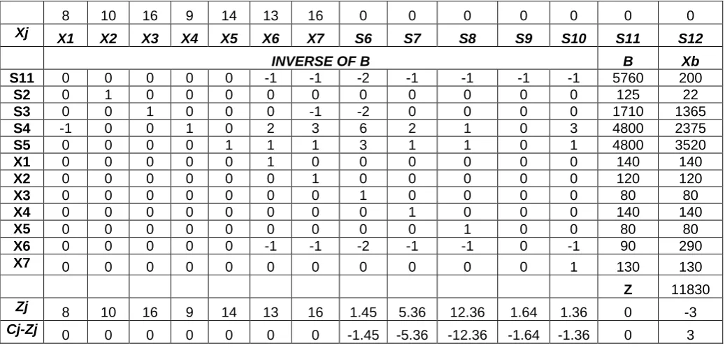
Table IX shows that the last row Cj-Zj in the tenth iteration all values are less than or equal to zero. Therefore, It is the last iteration and the optimal solution to the problem will be obtained. The variables in the base in addition to the 7 decision variables were: s11, s2, s3, s4 and s5 that correspond to the margin variable of equation 11 that expresses an excess in decision variable X6, in S2 the amount of resources that were allowed to be used, and with S3, S4 and S5, a smaller amount of time is used than the company owns. See table IX.
Table IX. Matrix identity base of the tenth iteration.
0 0 0 0 0 -16 -16 -16 -16 -16 -16 -16
Xj S1 S2 S3 S4 S5 A1 A2 A3 A4 A5 A6 A7
MATRIX B
S11 0 0 0 0 0 4 6.5 12 4.5 6.5 5.5 5.5
S2 0 1 0 0 0 0.07 0.11 0.16 0.1 0.13 0.1 0.11
S3 0 0 1 0 0 0 1.2 1.5 0.3 0 0 0.3
S4 0 0 0 1 0 1 2 2.5 1.5 3.5 4 1.5
S5 0 0 0 0 1 0.5 1 1.5 1 1.5 2 1
X1 0 0 0 0 0 1 0 0 0 0 0 0
X2 0 0 0 0 0 0 1 0 0 0 0 0
X3 0 0 0 0 0 0 0 1 0 0 0 0
X4 0 0 0 0 0 0 0 0 1 0 0 0
X5 0 0 0 0 0 0 0 0 0 1 0 0
X6 -1 0 0 0 0 0 0 0 0 0 1 0
X7 0 0 0 0 0 0 0 0 0 0 0 1
S11 S2 S3 S4 S5 X1 X2 X3 X4 X5 X6 X7
CB 0 0 0 0 0 8 10 16 9 14 13 16
ZJ 2.36364 0 0 0 0 -1.455 -5.364 -12.3636 -1.6364 -1.3636 0 3
The results and the objective value of the gain with the products analyzed can be seen in Table X. The final profit is $ 11830. The solution vector Xb gives the optimal solution respecting the limitations that we have. See Table X.
Table X. Matrix identity base of the tenth iteration.
8 10 16 9 14 13 16 0 0 0 0 0 0 0
Xj X1 X2 X3 X4 X5 X6 X7 S6 S7 S8 S9 S10 S11 S12
INVERSE OF B B Xb
S11 0 0 0 0 0 -1 -1 -2 -1 -1 -1 -1 5760 200
S2 0 1 0 0 0 0 0 0 0 0 0 0 125 22
S3 0 0 1 0 0 0 -1 -2 0 0 0 0 1710 1365
S4 -1 0 0 1 0 2 3 6 2 1 0 3 4800 2375
S5 0 0 0 0 1 1 1 3 1 1 0 1 4800 3520
X1 0 0 0 0 0 1 0 0 0 0 0 0 140 140
X2 0 0 0 0 0 0 1 0 0 0 0 0 120 120
X3 0 0 0 0 0 0 0 1 0 0 0 0 80 80
X4 0 0 0 0 0 0 0 0 1 0 0 0 140 140
X5 0 0 0 0 0 0 0 0 0 1 0 0 80 80
X6 0 0 0 0 0 -1 -1 -2 -1 -1 0 -1 90 290
X7 0 0 0 0 0 0 0 0 0 0 0 1 130 130
Z 11830
Zj 8 10 16 9 14 13 16 1.45 5.36 12.36 1.64 1.36 0 -3
Cj-Zj 0 0 0 0 0 0 0 -1.45 -5.36 -12.36 -1.64 -1.36 0 3
The result for the tank top is 140 garments, for the short sleeve blouse is 120, for the long sleeve blouse is 80, the basic boxer is 140, for the Fajilla is 80, Scarleth blouse is 290 and for the boxer with designs is 130.
V. CONCLUSIONS.
In this research paper a linear programming model was developed, using the revised simplex model in an Excel spreadsheet. Several visits were made to a textile SME to record data pertaining to each one of its manufacturing steps. Time cycle, inputs and demand constraints were implemented in each step. A gain of $11,830.00 MXN was obtained in the process. In the model there was no consideration of the quality control process. The simplicity of the revised simplex model allows to work in Excel spreadsheets, with the added portability in other economical activities. The results allowed the enterprise to take better decisions in the assignation of order priorities. Future works will design a neural network to predict the demand of its main products.
REFERENCES
[1] . OLIVA, J.C., “El sector textil-confección
español: situación actual y perspectivas”. Boletín económico de ICE, 2003, no 2768.
[2] OLIVOS, P.C., “Modelo de gestión logística para
pequeñas y medianas empresas en México. Contaduría y administración", 2015, vol. 60, no 1, p. 181-203.
[3] OROZCO, D.L, ARIAS, C.C., RODRÍGUEZ, C.
O., “Modelo para la evaluación de alternativas de
localización de una PTAR para una ciudad en el Valle del Cauca Colombia”. Scientia et technica, 2016, vol. 21, no 1, p. 43-50.
[4] CABALLERO, J. A., GROSSMANN, I. E., “Una
revisión del estado del arte en optimización. Revista Iberoamericana de Automática e Informática Industrial”, RIAI, 2007, vol. 4, no 1, p. 5-23.
[5] Sahinidis, N. V., “A general purpose global optimization software package. Journal of Global Optimization”, 8(2), 201-205.
[6] ACERO, L. M., “Aplicación de método simplex
para un modelo en la producción de leche y sus derivados en pequeños y medianos productores”, 2017.
[7] BURGOS, M. F., “Modelo de programación
matemática para la optimización de las utilidades bajo niveles de riesgo en una empresa de cultivo de langostinos del Perú”, 2012.
[8] INFANTE, R. A., “HERRAMIENTA PARA LA
OPTIMIZACIÓN DE FLUJOS METABÓLICOS EN UN SISTEMA BIOLÓGICO”, Investigación Operacional, 2014, vol. 35, no 2, p. 96-103.
[9] MÉNDEZ, R. E., “Planteamiento teórico para la
optimización del control mecánico de maleza en la infraestructura hidroagrícola de las zonas de riego. Revista de Ingeniería Hidráulica y Ambiental”, 2010, vol. 31, no 3, p. 28-32.
[10] AGREDA QUEZADA, L. A., “Aplicación del método simplex para maximizar los beneficios obtenidos por la fabricación de carrocerías en la empresa Éxito SA”. 2016.
[11] RODRÍGUEZ, N.P., “Método simplex secuencial para la optimización de sistemas con respuestas múltiples”, 2003. Tesis Doctoral. Universidad de Puerto Rico, Recinto Universitario de Mayagüez.