Enhancement Of Power Transfer Capability For IEEE Bus Systems By Using Power Flow Methods

e- ISSN: 2278-067X, p-ISSN: 2278-800X, www.ijerd.com

Volume 14, Issue 6 (June Ver. I 2018), PP.23-32

Enhancement Of Power Transfer Capability For IEEE Bus

Systems By Using Power Flow Methods

M.Sheshagiri

, Dr.B.V.Sanker Ram

1

Divisional Engineer, TSTRANSCO, Vidyut Soudha, Hyderabad, Telangana, India

2_{Professor, Department of Electrical and Electronics Engineering, College of Engineering Hyderabad, JNTUH,}

Telangana, India

Corresponding Author: M.Sheshagiri

ABSTRACT:- In order to facilitate the electricity market operation and trade in the restructured environment, ample transmission capability should be provided to satisfy the demand of increasing power transactions. The conflict of this requirement and the restrictions on the transmission expansion in the restructured electrical market has motivated the development of methodologies to enhance the Available Power Transfer Capability of the existing transmission grids. One of the conventional strategies is by inserting FACTS devices in electrical systems seems to be a promising strategy to enhance power transfer capability. In this paper, the work has been carried out on IEEE 14 bus system with different power flow methods like continuation power flow method, repeated power flow methods are employed to obtain the optimal settings for FACTS controllers and reducing losses, power balancing and control, reduce locational marginal price.

KEYWORDS:- Available Transfer Capability(ATC), Flexible AC Transmission Systems, continuation method, repeated power flow(RPF) methods, transient and steady state operations.

--- Date of Submission: 01-06-2018 Date of acceptance: 16-06-2018

---I. INTRODUCTION

The restructuring of the electric industry throughout the world aims to create competitive markets to trade electricity and generates a host of new technical challenges to market participants and power system researchers. For transmission networks, one of the major consequences of the non-discriminatory open-access requirement is a substantial increase of power transfers, which demand adequate available transfer capability (ATC) to ensure all transactions are economical. FACTS technology enables line loading to increase flexibly, in some cases, even up to the thermal limits.Therefore, it can theoretically offer an effective and promising alternative to conventional methods for ATC enhancement. Undoubtedly, it is very important and imperative to carry out studies on exploitation of FACTS technology to enhance ATC [7]-[9]. The modeling of FACTS devices for power flow studies, the role of such modeling for power flow control and the integration of these devices into power flow studies were reported in the literature [1],[2]. Modeling and the role of important

FACTS devices

like static VAR compensator (SVC), Thyristor controlled series compensator(TCSC) and unified power flow controller (UPFC) in solving power system restructuring issues have been previously reported [3]-[5]. Some well established search algorithms such as GA [1] and evolutionary programming (EP) [7], [8] were successfully implemented to solve simple and complex problems efficiently and effectively. Most of the population based search approaches are motivated by evolution as seen in nature. Particle Swarm Optimization (PSO), on the other hand, is motivated from the simulation of social behavior and was introduced by Eberhart and Kennedy [9].

II. ATC

An easy way to comply with the paper formatting requirements is to use this document as a template and simply type your text into it.

ATC is a measure of the transfer capability remaining in the physical transmission network for further commercial activity over and above the already committed uses. It can be expressed as follows:

ATC  TTC  Existing Transmission Commitments…(1)

using line flow limit (thermal limit) criterion is mathematically formulated using ACPTDF as given in the below equation:

ATCmn = min, T ij, mn i,j NL ...(2)

III. POWERFLOWMETHODS

The application of Optimal Power Flow (OPF) in power system congestion management has been studied by some researchers [6][7][1][2]. In the mean time, TTC calculation by OPF approach has been proposed since 1999 [3][4][5]. The basic concept of OPF approach is formulating the TTC calculation as an optimization problem, with equity constraints of power flow, inequality constraints from basic operation and equipment limits to more detailed approximation of transient stability security requirements. The objective function, obviously, is the maximum power flow on the specified transmission route. To determine the total transfer capability the objective is to maximize the power transfer between the two areas subjected to the conditions that there is no voltage or thermal or stability limit violations. Total transfer capability problem formulation can be explained as follows.

CONTINUATION POWER FLOW:

The general principle behind the continuation power flow is simple. It employs a predictor-corrector scheme to find a solution path. It adopts locally parameterized continuation technique. It includes load parameter, step length for load parameter and state variable.

Locally Parameterized Continuation

A parameterization is a mathematical means of identifying each solution on the branch, a kind of measure along the branch. When we say "branch," we refer to a curve consisting of points joined together in n + 1 dimensional space that are solutions of the nonlinear equations F(x , λ) = 0 (1). This equation is obtained by introducing a load parameter λ into the original system of nonlinear equations, F(x) = 0. For a range of values of λ. The solution of mathematical equations can be solved along a given path can be found for each value of λ, although problems arise when a solution does not exist for maximum possible λ value. At this point, one of the state variables, X can be used effectively as the parameter to be varied, choice of which is determined locally at each continuation step. Thus, the method is designated as the locally parameterized continuation. In summary, local parameterization allows not only the added load parameter, but also the state variables to be used as continuation parameters. Continuation power flow finds successive load flow solutions according to a load scenario.

From a known base solution, a tangent predictor is used so as to estimate next solution for a specified pattern of load increase. The corrector step then determines the exact solution using Newton-Raphson technique employed by a conventional power flow. After that a new prediction is made for a specified increase in load based upon the new tangent vector. Then corrector step is applied. This process goes until critical point is reached. The critical point is the point where the tangent vector is zero. The illustration of predictor-corrector scheme is depicted in Fig 1.

and without reactive power limit constrains. Continuation power flow is run up to bifurcation point, that means when maximum loading point reaches power flow will stop. Here distributed slack bus is used so all transmission losses distributed among all buses. At base case loading point lambda is taken 1 and load increasing at each bus proportional to base load.

In practice, it is possible to find the Thevenin’s equivalent of any system with respect to the bus under consideration. It is to be noted that the generations are rescheduled at each step of change of the load. Some of the generators may hit the reactive power limit. The network topology may keep changing with respect to the critical bus, with change in the loading, thereby reducing the accuracy of the method. This method works well in the case of an infinite bus and isolated load scenario.

Fig 1: Bus voltage versus Load Repeated Power Flow method:

At a specified hour with congestion free market schedule, the maximum value of ATC can be obtained using RPF method, as the name implies, finds TTC by successively solving a set of power flow problems. The demand at buyer bus, and the generation at the seller bus are increased in an increment step until any of the operating constraints’ violation. In this paper, the voltage limit, thermal limit and generation capacity limits are considered. Finally the ATC will be equal to TTC minus base load at sink bus which can be further useful to bilateral transaction.

The computational procedure of this approach is as follows: i. Establish and solve for a base case

ii. Select a transfer case iii. Solve for the transfer case

iv. Increase step size if transfer is successful v. Decrease step size if transfer is unsuccessful

vi. Repeat the procedure until minimum step size reached

IV. RESULTSANDANALYSIS

Selection of IEEE 14-bus system

Fig 2: Single Line diagram of IEEE 14 Bus system

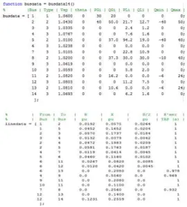
Identification of the line data, bus data

Fig 3: load flow line data and bus data (Without Reactive power Limits)

Fig 4: Load Flow using power flow Method (With Reactive power Limits)

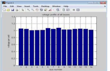
Fig 6: The voltage profile of all buses of the IEEE14 system as obtained from the load flow

Fig 7: Obtaining the minimum Eigen value

.Table 1: The value Eigen value associated of the reduced Jacobian matrix.

Mode Eigen value

1 74.7375 +23.0420i

2 74.7375 -23.0420i

3 67.9441 +18.4470i

4 67.9441 -18.4470i

5 36.0275

6 34.0436

7 27.7525 + 7.2245i

8 27.7525 - 7.2245i

9 23.6614

10 17.1925 + 0.4839i

11 17.1925 - 0.4839i

12 0.6486

13 1.6635

14 3.0627 + 1.0611i

15 3.0627 - 1.0611i

16 4.9664

17 6.0025

18 6.7607

19 7.4874

20 8.5508

21 9.6173

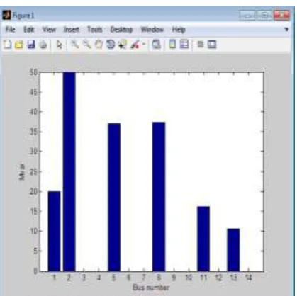
Fig 8: Margin of reactive power in IEEE 14 bus bar test system

Analysis:

Continuation power flow finds successive load flow solutions according to a load scenario. From a known base solution, a tangent predictor is used so as to estimate next solution for a specified pattern of load increase. The corrector step then determines the exact solution using Newton-Raphson technique employed by a conventional power flow. After that a new prediction is made for a specified increase in load based upon the new tangent vector. Then corrector step is applied. This process goes until critical point is reached. The critical point is the point where the tangent vector is zero.

Table 2: Transmission lines data (R, X and B in Pu on 100MVA base) for the 14-bus test system

End buses R X B/2

1-2 0.0192 0.0575 0.0264

2-4 0.0472 0.1983 0.0209

12-13 0 0.1400 0

Table 3: Transformer data in transmission line for tap setting (R, X in pu on 100 MVA base) for the 14-bus test system

Table 4: Shunt capacitor (R, X in pu on 100 MVA base) for the 14-bus test system for compensation

Table 5: Base case load data (Pu on 100 MVA base) for the 14-bus test system

End buses MVAR(pu)

4 0.191

5 0.016

End buses R X

3-8 0.0671 0.17173

7-9 0 0.11001

6-7 0 0.2522

Bus V(pu)

1 1.06

Table 6: Base case generator data (Pu on 100 MVA base) for the 14-bus test system

Table 7: Eigen values of reduced Jacobian matrix (Pu on 100 MVA base) for the 14-bus test system

Table 8: Transformer data for different load levels (Pu on 100 MVA base) for the 14-bus test system

End buses R X Tap setting

9-10 0.03181 0.08450

1 0.978 0.969 0.932

Table 9: Load data for different load levels (Pu on 100 MVA base) for the 14-bus test system

Bus P(pu) Q(pu) Load level

4 0.942 0.191 1

0.931 0.185 0.978

0.928 0.189 0.969

0.940 0.172 0.932

5 0.478 0.197 1

0.435 0.192 0.978

Table 10: Load voltages and reactive power outputs of generator 2 and 3 at load level 2 (Pu on 100 MVA base) for the 14-bus test system

Contingency V5 V6 QG3 QG2

Without outage, fixed tap 1.03 1.11 290 -83

Without outage, LTC active (Load

Level 2) 0.99 1.08 227 164

Without outage, LTC active (Load

Level 3) 0.98 1.07 700 249

Table 11: Voltage Sensitivity Factor of PQ Buses of IEEE 14 Buses at Base Case and Diff Contingencies

PQ Bus No VSF without RP limit VSF with RP limit VSF Line outage (2-3)

6 0.0929 0.2469 0.3388

9 0.0681 0.1594 0.2841

10 0.0969 0.2527 0.2763

12 0.0257 0.2295 0.3025

14 0.0409 0.2408 0.3152

Analysis: At the time of contingency case line outage (2-3) rank of most four weakest buses is changed, while for other contingency it remains same .Bus no. 6 is weakest bus in all contingencies cases. Above all results shows that voltage stability margin can be found easily by CPF. And P-V curve and max. Loading point can access. Only collapse point is not enough for voltage stability assessment .So, using tangent vector sensitivity analysis can be done. From voltage sensitivity factor weakest bus can identify. The Weakest bus identification is done by without excessive calculation. Placement of reactive power sources such as FACTS devices, capacitor bank can be inserted. From the comparison results CPF method is more accurate and simple for Voltage stability analysis but compensators can be easily placed by using RPF Method.

K E1 E2 E3 E4

Fig 9: Locational Marginal Price for the IEEE 14 system by using RPF method

Fig 10: Line flow data for IEEE 14-bus using RPF method

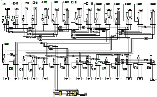
IEEE 30- Bus system (Case study):

The IEEE 30 Bus system is considered in estimation of TTC using different power flow methods. The 11 kV and 1.0 kV base voltages are considered as initial conditions. The model actually has these buses at either 132 or 33 kV.

Continuous

powergui

ABC abc ABC

abc

ABC abc ABC

abc ABC

abc ABC

abc

A BC A BC AB C AB C A BC A BC AB C AB C A BC A BC A BC A BC AB C AB C A BC A BC A BC A BC ABC ABC AB C AB C A BC A BC AB C AB C A BC A BC A BC A BC A BC A BC A BC A BC ABC ABC A BC A BC AB C AB C A BC A BC ABC ABC ABC ABC AB C AB C A BC A BC A BC A BC AB C AB C AB C AB C AB C AB C AB C AB C AB C AB C ABC ABC AB C AB C AB C AB C A BC A BC A BC A BC A BC A BC A BC A BC A BC A BC AB C AB C A BC A BC AB C AB C Sw Pulses A B C VdcP N VdcM Shunt Converter 500 kV, 100MVA

Pulses A1 B1 C1A2 B2 C2 VdcP N VdcM Series Converter 10% injection, 100MVA Scope9 Scope8 Scope7 Scope60 Scope6 Scope59 Scope58 Scope57 Scope56 Scope55 Scope54 Scope53 Scope52 Scope51 Scope50 Scope5 Scope49 Scope48 Scope47 Scope46 Scope45 Scope44 Scope43 Scope42 Scope41 Scope40 Scope4 Scope39 Scope38 Scope37 Scope36 Scope35 Scope34 Scope33 Scope32 Scope31 Scope30 Scope3 Scope29 Scope28 Scope27 Scope26 Scope25 Scope24 Scope23 Scope22 Scope21 Scope20 Scope2 Scope19 Scope18 Scope17 Scope16 Scope15 Scope14 Scope13 Scope12 Scope11 Scope10 Scope1

VabcAIabcBabCcBUS9 VabcIabcABabCcBUS8 VabcAIabcBabCcBUS7 VabcIabcABabCcBUS6 VabcIabcABabCcBUS5 VabcIabcABabCcBUS4

VabcAIabcBabCcBUS30 VabcAIabcBabCcBUS3

VabcIabcABabCcBUS29 VabcAIabcBabCcBUS28 VabcAIabcBabCcBUS27 VabcAIabcBabCcBUS26 VabcAIabcBabCcBUS25 VabcAIabcBabCcBUS24 VabcIabcABabCcBUS23 VabcAIabcBabCcBUS22 VabcIabcABabCcBUS21 VabcIabcABabCcBUS20 VabcAIabcBabCcBUS2

VabcIabcABabCcBUS19 VabcAIabcBabCcBUS18 VabcAIabcBabCcBUS17 VabcAIabcBabCcBUS16

VabcAIabcBabCcBUS15 VabcIabcABabCcBUS14 VabcAIabcBabCcBUS13 VabcAIabcBabCcBUS12 VabcAIabcBabCcBUS11 VabcAIabcBabCcBUS10 VabcIabc

ABabCcBUS1

VabcIabc PQ VabcIabc PQ VabcIabc PQ VabcIabc PQ VabcIabc PQ VabcIabc PQ VabcIabc PQ VabcIabc PQ VabcIabc PQ VabcIabc PQ VabcIabc PQ VabcIabc PQ VabcIabc PQ VabcIabc PQ VabcIabc PQ VabcIabc PQ VabcIabc PQ VabcIabc PQ VabcIabc PQ VabcIabc PQ VabcIabc PQ VabcIabc PQ VabcIabc PQ VabcIabc PQ VabcIabc PQ VabcIabc PQ VabcIabc PQ VabcIabc PQ VabcIabc PQ VabcIabc PQ abc Mag Phase abcMag Phase abcMag Phase abc Mag Phase abc Mag Phase abcMag Phase abcMag Phase abcMag Phase abcMag Phase abcMag Phase abcMag Phase abcMag Phase abcMag Phase abc Mag Phase abcMag Phase abcMag Phase abcMag Phase abc Mag Phase abc Mag Phase abc Mag Phase abcMag Phase abcMag Phase abc Mag Phase abc Mag Phase abc Mag Phase abc Mag Phase abc Mag Phase abc Mag Phase abc Mag Phase abcMag Phase

ABC

Gen6

ABC

Gen5

ABC

Gen4

ABC

Gen3

ABC

Gen2

ABC

Gen1

ABC

R Load 9

ABC

R Load 8

ABC

R Load 7

ABC

R Load 6

ABC

R Load 5

ABC

R Load 4

ABC

R Load 3

A B C R Load 26

ABC

R Load 25

ABC

R Load 24

ABC

R Load 23

ABC

R Load 22

ABC

R Load 21

ABC

R Load 20

ABC

R Load 2

ABC

R Load 18

ABC

R Load 17

ABC

R Load 16

ABC

R Load 15

ABC

R Load 14

ABC

R Load 13

ABC

R Load 12

ABC

R Load 11

ABC

R Load 10

ABC

R Load 1

Fig 12: Simulation model of IEEE 30-bus system

Fig 13: TTC for 30-bus system

Table 12: Enhancement of power transfer capability for IEEE 14-Bus system

From

Area To Area

TTC in MW

Constraint

OPF CPF RPF

1 2 36

36

42

Violating reactive power limit of generator at bus: 1;

3 2 44

48

53

Voltages at all buses are within permissible limits

1 5 43

45 50.2

Violating reactive power limit of generator at bus: 1;

Table 13: Enhancement of power transfer capability for IEEE 30-Bus system

From

Area To Area

TTC in MW

Constraint

OPF CPF RPF

25 26 115.9 115.1 168.1 Violating reactive power limit of

generator at bus: 26;

29 30 116.18 115.3 168.4 Violating reactive power limit of

generator at bus: 30;

V. CONCLUSIONS

source is increased. The results have been improved by using Repeated Power Flow (RPF) for the computation of transfer capabilities between system areas. A significant reduction in computational time, thus making it a potential candidate for online application. The work proposed in this paper can also be used to calculate available transfer capabilities (ATC) under the open access environment.

REFERENCES

[1]. Venkataramana Ajjarapu ―Computational Techniques for Voltage Stability Assessment and Control‖ E-Book— Library of

Congress Control Number: 2006926216 , Iowa State University ,Department of Electrical and Computer Engineering . 1122 Coover Hall ,Ames Iowa 50011, U.S.A.

[2]. Varun Togiti ―Pattern Recognition of Power System Voltage Stability using Statistical and Algorithmic Methods‖ University of

New Orleans ScholarWorks@UNOUniversity of New Orleans . 5-18-2012

[3]. B. Gao, G. K. Morison, and P. Kundur, ―Voltage stability evaluation using modal analysis,‖ IEEE Trans. on Power Systems, vol.

7, no. 4,pp. 1529–1542, Nov. 1992

[4]. P. A. Lof, T. Smed, G. Anderson, and D. J. Hill, ―Fast calculation of a voltage stability index,‖ IEEE Trans. on Power Systems,

vol. 7, no. 1,pp. 54–64, Feb.1992..

[5]. L. Bao, Z. Huang, and W. Xu, ―On-line voltage stability monitoring using var reserves,‖ IEEE Trans. Power Syst., vol. 18, no. 4,

pp.1461 –1469, Nov. 2003.

[6]. Satish Joshi , ―A Thesis on Voltage stability and contingency selection studies in electrical power system‖, Department of

electrical engineering. Indian institute of technology Kanpur . December 1995.

[7]. P. Kundur, ―Power System Stability and Control‖ McGraw-Hilll, 1994.

[8]. J. Paserba, V. Ajjarapu, G. Andersson, A. Bose, C. Canizares, N. Hatziargyriou, D. Hill, A. Stankovic, C. Taylor, T. Van Cutsem,

V. Vittal, P.Kundur, "Definition and Classification of Power System Stability," IEEE Trans. on Power Syst., vol. 19, no. 2, pp. 1387-1401, May 2004.

[9]. ―S. Kamel, M. Kodsi and C. A. Canizares, ―Modeling and simulation of IEEE 14 bus system with facts controllers‖, Technical Report, (2003), p. 3.‖