Variable Selection Method for Aluminum Electrolytic Process Based on FNN and RM in KPLS Feature Space

Variable Selection Method for Aluminum

Electrolytic Process Based on FNN and RM in

KPLS Feature Space

Lizhong Yaoa_{, Taifu Li}a_{, Jun Peng}a_{, Deyong Wu}b_{, Yingying Su}a_{, Jun Yi}a

a _{School of Electric and Information Engineering, Chongqing University of Science and Technology, Chongqing,} 40133,China

Email: [email protected]; [email protected]; [email protected]; [email protected]; b _{School of Materials Science and Engineering, Chongqing University of Technology, Chongqing, 400054,China}

Email: 279062432 @qq.com

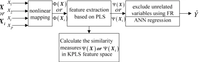
Abstract—Selecting the process variables is an important prerequisite for establishing an accurate model of aluminum electrolytic process. A variable selection method is researched and proposed based on the False Nearest Neighbors (FNN) and Randomization Method (RM) (FR) in KPLS(Kernel Partial Least Squares) feature space. Firstly, the KPLS is employed to transform the original space to the PLS feature space; secondly, in the new feature space, the FNN is used to calculate the similarity measure of each variable which first is retained and then reset to zero for evaluateing the importance to the dependent variable; then, the RM is utilized to test the significance level of the importance for each variable in turn, so the redundant variables would be excluded; lastly, technical energy consumption model of aluminum electrolytic process is built to verify the presented method. The experimental results show that the method selects out the best process variables of aluminum electrolytic process. Therefore, the research provides a new method of the variable selection for metallurgical industrial processes.

Index Terms—variable selection, aluminum electrolysis, false nearest neighbors(FNN), randomization method(RM), KPLS

I. INTRODUCTION

Aluminum electrolysis process has the multiple characteristics, which gather the multivariate, strong coupling, strong interference and the time-varying parameters in integral whole [1] [2]. When the model of aluminium electrolysis process is established, the complexity of the model will increase exponentially along with decision variables [3]. Thus, the accuracy and efficiency of the model can not be guaranteed. Therefore, how to choose the best combination of process variables is a very important part for establishing an accurate

technical energy consumption model in aluminum electrolytic process.

Traditional methods of variable selection such as forward selection [4], backward elimination [5], stepwise regression [6], ridge regression [7], bootstrap [8] and Partial Least-Squares Regression(PLSR) [9] couldn’t apply to selecting variables for nonlinear data, due to the nonlinear distortion of the image data in low-dimensional space [10].

The method of feature extraction based on kernel function is an effective way to eliminate information redundancy of the nonlinear variable [11]. It reduces the dimension of data by eliminating the linear correlation data, meanwhile，_{solves the problem of dimension}

disaster of high-dimensional data. The following method is often used, for instance， _{Kernel Principal Component}

Regression (KPCR) [12], Kernel Principal Component Analysis (KPCA) and neural networks [13], KPCA and Support Vector Machine (KPCA-SVM) [14], Kernel Fisher Fiscriminate Analysis (KFDA) [15], Kernel Independent Component Analysis and SVM (KICA-SVM) [16], etc. Unfortunately, the feature extraction just gets the combinations of original variables, and do not meet the purpose of reducing the number of process variables.

For exploring a way to overcome the above defects, we have done some research using the FNN method [10] [17]. Firstly, the initial nonlinear space is converted to linear space based on kernel function; then, the FNN is employed to calculate the similarity measure of the each variable by retaining and removing to determine the importance to the output variable. This approach provides a very important revelation for selecting out the best process variables. However, after further detailed research, we find that although FNN can quantify the important degrees of variables and provides the sorting of important degrees, it doesn't come up with a specific standard to filter out the best variables. Fortunately, randomization method (RM) is a pruning technique, which can test the significant level of statistical indicators based on statistical theory and then exclude no significant indicators [18].

Based on those reasons, A novel variable selection strategy is proposed based on the FNN and RM in Kernel

Manuscript received June 1, 2013; revised July 5, 2013; accepted July 12, 2013.

Spaces.Taking into account the partial least square (PLS) [19] having many advantages, which not only involves the relationship between independent variables, but also between the independent variable and dependent variable. So, the space of kernel partial least square (KPLS) [20] is used to participate in the process of selecting the best process variables.

II. PRELIMINARIES

A. Kernel Partial Least Squares(KPLS)

KPLS is a nonlinear PLS method combined with the kernel function and PLS. The most commonly kernel function is Gaussian kernelK x x



i, j



=exp(- xi xj 2/c), where c is a constant. So the feature subspace can be constructed to infinite dimension. Assuming the main component of the independent variable matrix is represented as t, the main component of the dependent variable matrix as u, the sample data in the original space _Rl n _{as X ,the variable dimension as}

n , the number of samples as l. After the nonlinear transform, it is mapped to high dimensional feature space H, where its’structure is lN (N n) and  is a matrix of n H , the i-th line is the vector 

 

x_i . The specific algorithm is presented as follow：

1) Initialize vector u randomly;

2) Calculate _{t }T_{u , Normalization tt/ t ；}

3) Independent variable spatial weight vector_{cY t}T _;

4) Calculate uYc, Normalization uu/ u ； 5) Repeat steps 2)—4), until convergence;

6) Calculate the residual space of the feature space and the dependent variable space, as in (1).







T

T _ttT _ttT

        ,_{Y Y tt Y}T ₍₁₎

Where: _T _{represents the nuclear matrix K ,}



i,

    

i j

T i

K x x  x  x .

B. False nearest-neighbor method(FNN)

FNN[17] is a method used to determine the input space dimension of autoregressive time series prediction model, belonging to the phase space reconstruction method. Assuming that the phase space is the m dimensions, where a phase point vector is denoted by

( ) { ( ), ( ), ,

X t  x t x t  x t( ( m1) )}, t1,2, , m , there must be a nearest neighbor point Xf in a distance,

and its distance is ( )R tm  X t( )Xf( )t .If the dimension of the phase space expand from m to m1, the two - point distance measure will change to:

R2₊₁( )t R2( )t x t( m ) x (t m )2

m  m     f   (2)

Through the above analysis,the importance of decision variables from two models f₁



x x₁, , , , ,₂ xi xd



and





2 1, , , , ,2 i d 1

f x x  x  x _ can be calculated by using FNN algorithm.According to equation (2),we can easily see that characteristics xd1 is or not important, depending on

the change (x tm)x tf( m) between the Rm( )t

and Rm 1 ( )t whether or not significant difference. If Xf

is used as the origin of the feature space,that ( ) (0,0, ,0)

f

X t   , the change (x tm)x t_f( m) between Rm( )t and Rm 1 ( )t has become xd1 .And then

according to the pthagorean theorem, calculating xd1 is

changed to calculate the euclidean distance between



x x1, , , ,2 xd xd1





A  and B



x x₁, , , ,0₂  x_d



.In actual applications, we use a similarity measure cos instead of (x tm)x tf( m) . In order to complete the investigation of all decision variables，_{specific steps}

are as follows：



x x1, ,, ,0, ,2 xd



  

B

AB

cos



x x

1 2

, ,, , , ,

x

i

x

d









A

Figure 1. The diagram of FNN

1) As shown in Fig.1, d-dimensional data which is composed by all decision variables is viewed as



x x1, , ,2 xd





A  .

2) Remove the original decision variables xi ,we can

get a low-dimensional space projection , as in (3). B



x x1, ,2xi1,0,xi1, , xd



(3)

3) Calculate the similarity measure cosAB between the

high-dimensional phase space point A and its projection B.

Where: A BT A B AB

cos = 

 (4)

4) Examine variables x x1, , ,2 xd in turn, determine

the influence of the input variables to the original data structure by comparing the corresponding change of

1

l

i AB cos 



, and sort according to the change from big to small in the last，_where l is the number of samples.

The greater the similarity measure cosAB ，and the

smaller the effect to the original data structure when removing the variable;however, the smaller the similarity measure cosAB , the larger the to the original data

C. Randomization method(RM)

RM [18] is a pruning technique essentially, which do count test significantly of statistical indicators based on

the statistical theory, excluding no significant indicators, and then retaining significant indicators, so achieving the

purpose of excluding irrelevant variables. .

   

 X or Xi

1

x

2

x

i

x

p

x or

X

i X

   X

or

   Xi

 

 X or  

 Xi

ˆ Y

Figure 2. The diagram of decision variable selection based on FR in KPLS feature sapce

In order to make variable importance obtained by FNN more statistical significance, using RM to test the significant level of the variable similarity measures and exclud irrelative variables is an effective way.

Therefor, under the revelation of the RM and FNN, similarity measure of input variables based on FNN as shown in the formula (4) is used to do a random test.Finally,the decision variables can be selected according to the high and low of the significant level. Following these steps:

1) According to a large number of data samples normalized, calculate the similarity measure of each decision variable using FNN, and refer to as the standard value.

2) Randomly change the order of the sample output set.

3) Used the new samples and FNN, recalculate the similarity measure of each decision variable and record as the random value.

4) Repeat steps 2) and 3) a large number of times, using count to record the number of repetitions(such as 999), according to the step 3)to record every random value.

5) Calculate the significant degree P of similarity measure for each decision variable .

a)If the standard value is greater than 0,

( 1) / ( 1)

P N COUNT , N is the number of the random value greater than or equal to the standard value.

b)If the standard value less than 0,

( 1) / ( 1)

P M COUNT , M is he number of the randomization value less than or equal to the standard value.

6) If P is less than or equal to the significant level  (such as 0.05), reserve the decision variable, otherwise exclude.

III. THE PROPOSED METHOD

In this section, we describe the proposed variable selection algorithm based on FR in KPLS feature space. A. The Basic Principles of FR

The basic principles of FR: any variable xi in the

original variable group X( , , , ,x x1 2  xi xn) is set to

zero using FNN, and get a new variables set

1 2

( , , ,0, ) i x x xn

X   . Then the two points are

mapped to feature space by the kernel function and the similarity measure cos between two points can be calculated in the new space. All the cosi(i1,2, , n)

are arranged from small to large order, and the original variable which has greater similarity measure indicates it has little contributions to dependent variable. Finally, the RM is used to test the significant level of similarity measure from each variable. If a variable has not significant meaning, then it can be deleted from variables set. The diagram is showed in Fig. 2.

B. The Variable Selection Algorithm

Based on the above analysis, the variable selection algorithm based on FR in KPLS feature space can be described as follow:

1) The KPLS algorithm

Input:dataX{ , , }x₁ xl ,dimensionn;

1

{ , , }y yl



Y  ,dimensionm; a) Initialize vector urandomly; b) _{t }T_{u,tt/ t ;}

c) _{cY t}T _;

d) uYc,uu/ u ;

e) Repeat steps b)—_{d), until convergence;}

f) Calculate the residual space of the feature space and the dependent variable space







T

T _ttT _ttT

        ,_{Y Y tt Y}T ₍₅₎

Where _{K }T_,



_,

    

i i j

T i

K x x  x  x .

Output：_{Transformed data} Xˆ _{{ , , }}xˆ₁ xˆ_l . 2) FR algorithm

a) for i1:n for j1:l

Calculate the similarity measure of i-th variable in column j before and after set to zero:

(:, ) (:, ) (:, ) (:, )

T ij

A j B j cos

A j B j

  

 (6)

end

TABLE I.

DAILY DATA FROM 11 KINDS OF PROCESS PARAMETERS

z x1 x2 x3 x4 x5 x6 x7 … x11 Y

1 1751 2.55 16.6 17 945 1236.4 19 … 1250 12245

2 1750 2.55 16.3 18 944 1240 20 … 1250 12320

3 1744 2.55 17 15 946 1236 17 … 1240 12268

4 1745 2.59 18 16 947 1231.5 18 … 1220 12558

… … … …

130 1682 2.44 18 14 951 1236.5 15.4 … 1210 11905

TABLE II.

SIX PRINCIPAL COMPONENT SCORES EXTRACTED BY KPLS

the data sample from aluminum electrolytic process

C l₁ l₂ l₃ l₄ l₅ l₆ l₇ l₈ … l₁₃₀

1

C 1.012 0.058 0.129 -0.046 0.233 0.342 -.237 0.239 … 0.001

2

C 0.149 0.351 -0.829 0.377 -0.345 0.339 0.480 -0.029 … -0.065

3

C -0.008 0.577 0.187 0.577 0.546 0.558 0.677 0.1568 … 0.078

4

C 0.512 -0.34 0.135 -0.34 0.435 0.114 -0.042 0.154 … 0.146

5

C 0.289 0.671 -0.569 0.897 -0.446 0.219 0.202 -0.933 … -0.214

6

C 0.438 0.472 0.452 0.384 0.721 -0.35 0.523 0.677 … 0.084

i-th variable :

cos 1 n₁ i _j cos ij

l

 



_  (7)

end

Recorde the average of the similarity measure as the standard value(before randomized). .

b) Randomly change the order of the sample output set;

c) Repeat steps a) and b),and using COUNT to record the number of repetitions (such as 999), according to the step a)to record every random value;

d) Calculate the significant degree P of similarity measure for each decision variable;

① _{If the standard value is greater than 0,}

P(N1) / (COUNT1) (8) then Nas the randomization value greater than or equal to the number of standard values;

② If the standard value less than 0,

( 1) / ( 1)

P M COUNT (9) M is he number of the randomization value less than or equal to the standard value.

e) If P is less than or equal to the significant level  (such as 0.05), reserve the decision variable, otherwise exclude.

According to significant indicators of n variables, the decision variable whose significant level 0.05 will be excluded from the variables set. The original

variable group is T

1 2

( , , , )x x xn



X  , and the new set of independent variables after excluding redundant variables is Xˆ ( , , , )x xˆ ˆ_{1 2}  xˆk which reduces n k

dimensions.

IV. SIMULATION EXPERIMENTS AND RESULTS ANALYSIS

A. Variable Selection of Aluminum Eelectrolytic Process The nonlinear data set used in the experiment research is collected from the actual production site of aluminum reduction cell. Parameters are respectively in detail line current(A) represented x1 ,molecular ratio(1)

2

x , aluminum level(cm) x₃, electrolyte levels(cm) x₄, cell temperature

 

o_C

5

x , aluminum tapping volume (kg)

6

x , daily dosage of fluoride salt (kg) x₇ , blanking interval (s) x8, cell voltage(mv) x9,blanking times(1)

10

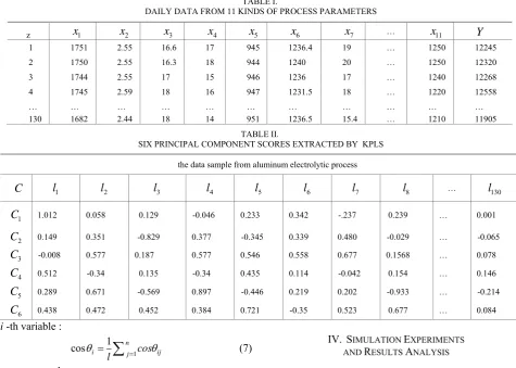
x , aluminum indicator(kg) x₁₁, aluminum electricity consume per ton ( KW h t Al  )Y .By sampling the electrolyzer No. 224 which is 170KA series from an aluminum factory, we've collected the 130 group daily data from 11 kinds of process parameters，_{as shown in}

Table I.

By applying the method proposed in combination with parameter matrixs from Table I，_{six principal}

component scores C C C C1, , ,2 3 4, ,C C5 6 can be easily

calculated and extracted by KPLS, as shown in Table II. Then, the x x1, , ,2 x11 are projected into a new

space built byC C C C₁, , ,_{2 3 4}, ,C C_{5 6},Y . The FR is used to calculate the similarity measure of each process variables in the new space. For instance, x1 from in

TABLE III.

THE AVERAGEOF SIMILARITY MEASURE AND SIGNIFICANT INDICATORS BASED ON FR IN KPLS FEATURE SPACE

i

x x₁ x₂ x₃ x₄ x₅ x₆ x₇ x₈ x₉ x₁₀ x₁₁

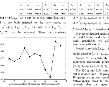
asm 0.693 0.656 0.697 0.846 0.723 0.766 0.742 0.536 0.426 0.942 0.878



0.043 0.024 0.032 0.026 0.05 0.042 0.032 0.014 0.004 0.572 0.736

vectorb= 0



,x2,,x11



can be gotten. After that, the a

and b are both mapped to the new space, so the a = C



1a C2a C11a Y



* _{, , , , and}



1 2

b = Cb Cb

* _{, ,}



11b C Y

, , _{can be obtained. Then the similarity}

0 2 4 6 8 10 12

0.4 0.5 0.6 0.7 0.8 0.9 1

decision variables of aluminum electrolytic process

the

av

er

age

of

s

im

ilar

ity

m

ea

su

re

m

en

t

Figure 3. The average similarity measure of process variables in aluminum electrolytic process

measure _{cosa b}* * _{can be calculated of a}* _{and b}*_.In accordance with the above procedures, the _{cosa b}* * _of

process variables can be gotten respectively. And then the average of similarity measure(asm) and the significant indicator ( =0.05) of each variable can be calculated and obatined, as shown in Table III. The Fig 3 shows thex10,x11 have the highest similarity measure.

Bold italics in the table indicate the corresponding variable has a significant effect, which must be retained, and the rest removed. So the variables x10,x11 will be

removed from the variables set. Finally



1, , , , , , , ,2 3 4 5 6 7 8 9 10 11



X  x x x x x x x x x， ，x x has become



1, , , , , ,2 3 4 5 6

X  x x x x x x x x x₇, ,_{7 9}



.

B. Model Analysis Based on ANN

In order to detailed analysis the precision and effect of the model before and after the variables removed, this study establishes two different models based on significant indicator  .

Model 1: exclude



x10,x11



,establish the mathematical

model based on



x x x x x x x x x1, , , , , , , ,2 3 4 5 6 7 8 9



.

Model 2: establish the mathematical model of aluminum electrolytic process based on all variables



x x x x x x x x x x1, , , , , , , , , ,2 3 4 5 6 7 8 9 10 x11



.

The 130 group daily samples of aluminum reduction cell is divided into 100 group training set samples and 30 group testing set samples. Then, the BP Neural Network[21]is used to build a 3-layer feedforward network, that the input of the decision-making parameters is 9 and 11 respectively, the output is aluminum electricity consume per ton, transfer function of the hidden layer and the output layers is sigmoid and purelin respectively. The formula (10) is used to determine the number of hidden nodes. The initial weights and biases of the artificial neural network(ANN) are set to the random number between (-1,1).

h n m k (10) Where: h is the number of hidden layer neurons; n the number of input layer neurons; m the number of output layer neurons; k the constant between 1-10.

After tested based on the formula (10)，_{the model 1}

employs 12 hidden layer nodes, and the model 2 employs 13. The model structure is shown in Fig. 4 from model 1 and Fig.5 from model 2. .

line current

molecular ratio

aluminum level

electrolyte level

cell temperature aluminum tapping volume

daily dosage of fluoride salt

blanking interval

cell voltage

H1 H2 H3 H4 H5 H6

H7 H8 H9 H10 H11 H12

KW.h/t-Al

line current molecular ratio aluminum level electrolyte level cell temperature aluminum tapping volume daily dosage of fluoride salt blanking interval cell voltage blanking times aluminum indicator

H1

H2

H3

H4

H5

H6

H7

H8

H9

H10

H11

H12

H13

KW.h/t-Al

Figure 5. Model 2

0 10 20 30 40 50 60 70 80 90 100 1.1

1.15 1.2 1.25 1.3 1.35 1.4 1.45x 10

4

Training samples

KW.

h/t

-A

l

the real value Model 1 Model 2

Figure 6. Fitting curve of the two models from the training set

0 5 10 15 20 25 30

1.1 1.15 1.2 1.25

1.3x 10

4

Testing Samples

C

at

eg

or

y La

be

ls

真真真 模模1

模模2

Figure 7. Fitting curve of the two models from the test set

TABLE IV.

Relevant statistical indicators from test set

Model Max Min Average MSE running time of model

Model 1 50 1 8 415 1.920

Fig. 6 and Fig. 7 are respectively the fitting curves of the training sets and test sets from the two models .Although both models get a good fitting effect from fitting curve which can be presented in Fig.6, the model 1 has a better fitting curve compared to the model 1, which can be seen clearly in Fig. 7. Meanwhile, according to the Table IV, it’s easy to find that the moel 1 not only has a higher precision, but also higher efficiency. Therefore, the model 1 which selects out the best process variables achieves a better effect after removing redundant variables.

V. CONCLUSION

In order to select out the best process variables of the energy consumption model in aluminum electrolysis process, a novel method based FR in KPLS feature space is presented. Firstly, he KPLS is employed to transform the original space to the PLS feature space; then, in the new feature space, the FNN is employed to calculate the similarity measure of process variables, so the importance rank of process variables can be obtained; lastly, the RM is used to test the significance level of the importance of each variable in turn, so the unrelated variables can be excluded. The results show that the process energy consumption model in aluminum electrolysis process obtains a high degree of accuracy after the edundant variables excluded.

In the future, the study will continue to explore the selective ability of FR in KPCA, KICA and KCCA feature space for forming a complete set of variable selection techniques and giveing the criteria of application of each method.

ACKNOWLEDGEMENTS

The work is supported by National Natural Science Foundation of China (No.51075418), Application Development Major Projects of Chongqing (No.cstc2013yykfC0034), Natural Science Foundation Key Project (No.CQ CSTC2013jjB40007), Chongqing Educational Committee Science and Technology Research Project (No.KJ111417 and No.KJ091402), Foundation of Chongqing University of Science and Technology (No. CK2011B04 and CK2011Z01).

REFERENCES

[1] G. Huchet, M. Boussuge, V. Maurel, H. Roustan, “Mechanical properties of a spinel-ferrite-based cermet: effects of temperature and oxidation,” Journal of Materials Science, Springer, vol.48,no.8,pp. 3264-3271, 2013 [2] C.-Y. Cheung, C. Menictas, J. Bao, M. Skyllas-Kazacos,

and B. J. Welch, “Spatial temperature profiles in an aluminum reduction cell under different anode current distributions,” American Institute of Chemical Engineers, Wiley-Blackwell, vol.59,no.5,pp. 1544–1556, 2013 [3] M. Abbasi, M. A. Abduli, B. Omidvar, A. Baghvand,

“Forecasting municipal solid waste generation by hybrid support vector machine and partial least square model,” International Journal of Environmental Research, Univ Tehran,vol.7, no.1,pp. 27-38,2013.

[4] R. D. Pereira, J. Sousa, S. Vieira, S. Reti, S. Finkelstein, “Modified Sequential Forward Selection Applied to Predicting Septic Shock Outcome in the Intensive Care Unit,” in Soft Methods in Probability and Statistics 2013, 2013 6th International Conference on,vol.190,2013,pp. 469-477

[5] K. Y. Chan, C. K. Kwong, T. S. Dillon, Y. C. Tsim, “Reducing overfitting in manufacturing process modeling using a backward elimination based genetic programming,” Applied soft computing, Elsevier, vol.11, no.2, pp. 1648-1656, 2011.

[6] N. Zhou, J. W. Pierre, D. Trudnowski, “A Stepwise Regression Method for Estimating Dominant Electromechanical Modes,” Power Systems, IEEE Transactons on, vol.27, no.2, pp. 1051-1059, 2012.

[7] F. Zhdanov, Y. Kalnishkan, “An identity for kernel ridge regression,” Theoretical Computer Science, Elsevier, vol.473, no. SI, pp. 157-178, 2013.

[8] C. X. Wu, J. K. Zhu, D. Cai, C. Chen, J. J. Bu, “Semi-Supervised Nonlinear Hashing Using Bootstrap Sequential Projection Learning,” Knowledge andData Enineering, IEEE Transactons on, vol.25, no.6, pp. 1380-1393, 2013. [9] J. C. Boulet, D. Bertrand, G. Mazerolles, R. Sabatier, “A

family of regression methods derived from standard PLSR,” Chemometrics and Intelligent Laboratory Systems, Elsevier, vol.120, pp. 116-125, 2013.

[10]J. Yi, T. F. Li, Y. Y. Su, W. J. Hu, T. Gao, “A variable selection method based on KPCA and FNN for nonlinear system modeling,”in BMEI, 2011 Proceedings IEEE , May 2011, pp. 832-835.

[11]J. B. Li, H. J. Gao, “Sparse data-dependent kernel principal component analysis based on least squares support vector machine for feature extraction and recognition,” Neural Computing& Applications, Springer, vol.21, no.8, pp. 1971-1980, 2013.

[12]R. C. Zhang, L. H. Wang, S. H. Zhang, “Windows memory analysis based on KPCR,” in Information Assurance and Security 2009, 2009 5th International Conference on, vol.2, 2009, pp. 677-680

[13]J. S. Wang, Q. P. Guo, “D-FNN based soft-sensor modeling and migration reconfiguration of polymerizing process,” Applied Soft Computing, Elsevier, vol.13, no.4, pp. 1892-1901, 2013.

[14]W. Suphamitmongko, G. L. Nie, R. Liu, “An alternative approach for the classification of orange varieties based on near infrared spectroscopy,” Computers and Electronics in Agriculture, Elsevier, vol.91, no.2, pp. 87-93, 2013. [15]J. H. Li, P. L. Cui, “Improved kernel fisher discriminant

analysis for fault diagnosis,” Expert Systems with Applications, Elsevier, vol.36, no.2, pp. 1423-1432, 2009. [16]Z. X. Li, X. P. Yan, C. Q. Yuan, “Intelligent fault

diagnosis method for marine diesel engines using instantaneous angular speed,” Journal of Mechanical Science and Technology, Korean Soc Mechanical Engineers, vol.26, no.8, pp. 2413-2423, 2012.

[17]H. D. Abarbane, R. Brown, J. J. Sidorowich, “The Analysis of Observed Chaotic Data in Physical Systems,” Rev. Mod. Phy., American Physical Soc, vol.65, no.4, pp. 1331–1392, 1993.

[18]J. D. Olden, D. A. Jackson, “Illuminating the ‘‘black box’’: a randomization approach for understanding variable contributions in artificial neural networks,” Ecological Modelling, Elsevier, vol.154, no.1-2, pp. 135-1502, 2002. [19]P. Susanne, K. Daniel, H. Thomas, “Significant amino

Science and Technology, Elsevier, vol.51, no.2, pp. 423-4322, 2013.

[20]N. Hadi, F. Abbas, N. Mehrab, “Application of GA-KPLS and L-M ANN calculations for the prediction of the capacity factor of hazardous psychoactive designer drugs,” Medicinal Chemistry Research, Springer, vol.21, no.9, pp. 2680-2688, 2012.

[21]J. J. Wang, B. L. Chen, Y. C. Yang. Mehrab, “Approximation of algebraic and trigonometric polynomials by feedforward neural networks,” Neural Computing& Applications, Springer, vol.21, no.1, pp. 73-80, 2012.

Lizhong Yao received his B.S. degree in automation from

Chongqing University of Science and Technology, China in June 2009 and his M.S. degree in Detection Technology and Automatic Equipment from Xi’an Shiyou University, China in June 2013. His current research interest includes modeling and optimization of complex systems.

Taifu Li received his B.Sc, M.Sc and Ph.D all from Chongqing

University in 1996, 2000 and 2004 respectively. Now he is a professor and supervisor for M.Sc candidate in Chongqing University of Science and Technology. His main areas of interest and research are intelligent control and soft-sensing.

Jun Peng received his Ph. D. degree from Chongqing

University, China in 2003. Now he is a professor and president in Chongqing University of Science and Technology. His main areas of interests are application of chaos theory and digital picture processing.

Deyong Wu received his B.Sc, M.Sc from Wuhan University

of Science and Technology, China in 2011. Now he is a Master degree candidate in Chongqing University of Technology. His main areas of interest is materials science.

Jun Yi received his Ph. D. degree from Chongqing University,

China in 2010. Now he is an associate professor at the Department of Electrical and Information Engineering, Chongqing University of Science and Technology. He His research interest includes intelligent control and wireless sensor network.

Yingying Su received her B.Sc and M.Sc from Heilongjiang