Improving the Spacecraft Center of Mass Stabilization Accuracy

ISSN (e): 2250-3021, ISSN (p): 2278-8719

Vol. 07, Issue 06 (June. 2017), ||V1|| PP 07-14

Improving the Spacecraft Center of Mass Stabilization Accuracy

Nickolay Zosimovych

Abstract: - The publication suggests how to significantly improve the spacecraft center of mass movement stabilization accuracy in the active phases of trajectory correction during interplanetary and transfer flights, which in some cases provides for high navigation accuracy, when rigid trajectory control method is used.

Keywords: - Space probe (SP), stabilization controller (SC), on-board computer (OC), gyro-stabilized platform (GSP), propulsion system (PS), angular velocity sensor (AVS), operating device (OD), space vehicle (SV), feedback (FB), control actuator (CA), control system (CS), angular stabilization (AS), center of mass (CM).

I.

INTRODUCTION

In some cases, when using a control system built according to the principle of program control (the "robust trajectories" method) the efficiency of task solution is much influenced by the accuracy of the spacecraft stabilization system in the powered portion of flight. This concerns, for example, the trajectory correction phases during interplanetary and transfer flights, when the rated impulse execution errors during trajectory correction resulting from various disturbing influences on the spacecraft in the active phase, greatly affect the navigational accuracy. Hence, reduction of the cross error in the control impulse on the final correction phase during the interplanetary flight, facilitates almost proportional reduction of spacecraft miss in the "perspective plane". For example, in some space probes (SP) like Deep Impact [1, 2] and Rosetta missions [3, 4] reduction of cross error by one order during the execution of correction impulse (for modern stabilization systems this value shall be 0.5 m/s) results in reduction of spacecraft miss in the "perspective plane" from 200 to 20 km. Such reduction of the miss accordingly increases a possibility of successful implementation of the flight plan, as well as the accuracy of the research and experiments conducted [5].Objectives: to solve the task of significant increase in stabilization accuracy of center of mass tangential velocities during the trajectory correction phases when using the "rigid" trajectory control principle.

Subject of research: The center of mass movement stabilization system in the transverse plane, which is used during the trajectory correction phases.In order the control actions could be created during the spacecraft trajectory correction phase, a high-thrust service propulsion system with a tilting or moving in linear direction combustion chamber shall be used.

II.

STATEMENT

OF

THE

PROBLEM

Improvement of control accuracy increases chances for successful implementation of the flight program. However, a significant reduction in the correcting impulse lateral error leads to reduction in fuel required for corrections, and thus increases the payload [5, 6]. The publication addresses spacecraft which use high- thrust PS for correcting impulses and control at active phases. During the active phase, the spacecraft shall be exposed to disturbances caused mainly by working PS. These disturbances create components of the spacecraft center of mass velocity in the normal and lateral directions (the drift velocity), and the spacecraft center of mass stabilization system is to provide center of mass lateral drift velocities close to zero during active phases. Since the time of the active phase T, which is determined by specified velocity impulse is not known and quite limited during correction maneuvers [7, 8] and in view of the fact that a guaranteed approach evaluating accuracy is always used to solve a guidance task in practice, in this publication, we shall understand the maximum dynamic error of the transition process  

max max z

y  with normal (lateral) drift velocity of the

III.

SYNTHESIS

OF

STABILIZATION

ALGORITHMS

IN

THE

SYSTEM

CONTROLLING

ROTATIONS

OF

THE

OPERATING

DEVICE

We study motions of the spacecraft in the normal plane of the inertial coordinate system XOY (Fig. 1)

[5]. The center O of the inertial coordinate system at the beginning of the active phase is the same as the center of mass of the spacecraft; the axis OX coincides with the direction of the required correction impulse V_cor,





axis OY together with axis OX form a normal plane. The angular position of the spacecraft in the normal plane is determined by an angle  between axis OX of the inertial coordinate system and X- axis O_cX_c of the bound

coordinate system. Control of the spacecraft in the active phase shall be done by deflection of combustion chamber of PS at an angle  between X-axis

c cX

O of the spacecraft and X-axis of the nozzle symmetry of PS.

Fig. 1. Spacecraft diagram in the inertial coordinate system

The following assumptions and conditions were used in the process of synthesis of the stabilization algorithms [5]:

1.We assume that the spacecraft is subject to disturbances in the active phase (force F and moment M ), which are mainly caused by working PS (tilt and thrust misalignment). Because of their nature, these parameters shall slowly change in time throughout the active phase (except for the period from the start of PS till switching to the nominal operation mode  0.2s). For this reason, the disturbances may be considered permanent within the active phase with a reasonable degree of accuracy: F const ;M const . We shall consider the work of the stabilization system within the entire possible range of disturbances:

max max ;0

0 F  F  M  M (experience shows that the maximum force and moment are respectively about

0.30 and 3.50 in the equivalent deviation angles of PS).

2.The motion of the spacecraft is considered as movement of the absolute rigid body in vacuum relative to the reference trajectory in the normal plane of the inertial coordinate system.

3.A high-thrust chemical engine is used to control the spacecraft in the active phase. Control is provided by deflecting PS combustion chamber. The servo control, which deflects the combustion chamber includes a feedback control actuator.

To stabilize the angular position of the spacecraft we shall use the information about deviation of the spacecraft body-fixed axes from the axes of the inertial coordinate system implemented in the gyro stabilized platform (CST) on board the spacecraft and the angular velocity sensors (AVS). The information on the deviation of the tangential velocities shall be taken from the accelerometers installed on CSP.

IV.

MATHEMATICAL

MODEL

OF

THE

SPACECRAFT

OF

MASS

MOTION

STABILIZATION

SYSTEM

Taking in consideration the above assumptions and suppositions we can set down a system of equations (1) describing the behavior of the spacecraft center of mass motion stabilization system under study:

    

  

 

  

),

(  



 

 

  

FB CM AS CA

z y y y

K y W W K

M C

F C C y

 

   

(1)

where y is the center of mass drift coordinate in the inertial coordinate system; C_y,C_y,C_  are dynamic

coefficients of the spacecraft; ,

m P C

C_y  _y  where P is PS thrust, m is mass of the spacecraft;

,

z

I Pl

C  where l is the distance from the gimbal assembly of PS to the center of mass of the spacecraft,



z

a velocity performance index of the control actuator; K_FB  is a control actuator feedback index; WAS  is a

response function of the angular stabilization controller; W_CM  is a response function of the stabilization

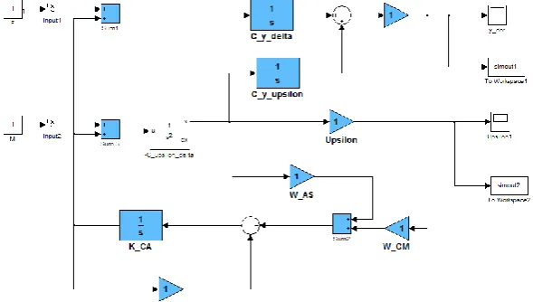
controller through the center of mass channel.According to the above mathematical model, a block diagram of the stabilization system under study shall be as follows (Fig.2) [5].In order to improve accuracy of stabilization while using synthesized algorithms, a model of a model of a standard stabilization system shall be made. It is to be used as a reference model for comparison. The standard stabilization model uses a known stabilization controller [8-10], which provides control proportionally to the angle , of the spacecraft angular rotation velocity in the normal plane , linear drift y and the drift velocity y. A block diagram of the standard stabilization system is shown in Fig. 3 [5].

Fig. 2. Block diagram of the spacecraft center of mass motion stabilization system under study

Fig. 3. Block diagram of a standard center of mass motion stabilization system of a spacecraft

V.

METHOD

TO

SOLVE

AN

INVARIANT

PROBLEM

VI.

PHYSICAL IMPLEMENTATION OF A STABILISATION SYSTEM

INVARIANT TO THE DESTABILIZING FORCE AND TO THE DISTURBING MOMENT

Let's consider the system of equations (1), which describes the system to be explored, the stabilization and the functional diagram (Fig 2) [5] in terms of the choice of response functions W_AS(s),W_CM (s) and

), (s

KFB providing invariance for coordinates y under influence F andM . The values F and M cannot be measured directly as supposed in combined regulation systems.

To analyze invariant conditions, we shall write equations (1) in operator form:

                          , 0 ) ( ) ( ) ( 2          CA FB AS CM y y K s s K s W y s W M C s F C C y s   (2)

According to the basic provisions of the invariant theory [13-15] it is necessary that (2) to ensure invariance y under influences F and M

0      

 yM yF

y

 

 (3)

Whence y_M  y_F  0, where y_M,y_F are invariant minors, and  is the main determinant of the

closed system (2).

By substituting the determinants y_M,y_F in (3) and  from the equations (2) we shall have the following necessary invariance conditions in the operator form [21]:

                             0 1 0 1 2    y AS CA FB AS CA FB C W s K K C C W s K K s (4) whence . , CA FB AS K s K

W 

 (5)

Rather than focusing so far on the meaning of the conditions obtained, let's consider the physical implementation of an invariant system providing the condition (4).We know that the requirement to ensure the open system's absolute invariance is a criterion for the physical implementation of the invariant system proposed by academician B. Petrov [22].

The expression for _OS shall be as follows [21]:

. 1 2                 

 s W C_

K K s s AS CA FB

OS (6)

It is easy to see that when conditions (5) are met, the expression (6) identically becomes zero, whence it follows that an absolutely invariant in moment M and force F system can't be implemented [21].Let's consider physical implementation of the system for each of the disturbances individually.

VII.

PHYSICAL IMPLEMENTATION OF A STABILIZATION

SYSTEM, WHICH IS INVARIANT UNDER DISTURBING MOMENT

0 

y_M is met, that is

. 0 1            _

 AS y

CA FB

y s W C

K K

C (7)

It is obvious that in general the expression (6) doesn't become zero in case the invariance condition (7) is met, which makes it clear that the condition for physical implementation of the center of mass stabilization system under disturbance M is met.

We shall demonstrate that the transfer function of the open system under disturbing moment M is equal

              s K K W C s C C s CA FB AS y y OS 1 0

0 2 _

 

(8)

The invariance minor ₂₁ shall be obtained by cancellation of the first column and the second line in (8):

. 1

1

21  

  y AS CA FB y CA FB AS y y C W s K K C s K K W C C                        

 (9)

The open system transfer function shall be as follows under disturbing moment M :

. ) ( ) ( ₂₁ OS M W s M s y      (10) Because 21

 meeting the invariance conditions (7) is zero, and ₂₁ is a minor of absolute invariance, so W_M 0, and therefore yW_MM 0. It is not possible to achieve a minor value ₂₁ exactly equal to zero, that is the actual value obtained y can be only close to zero [21]. It is significant that if the equality

, 0     _  y y C

C and therefore the equality   , are fulfilled, there are two channels for transmission of the

same disturbance M in the stabilization object itself, as can be seen from the block diagram (Fig. 3) [5] since



 y

y C

C  achieves absolute invariance under M .

VIII.

PHYSICAL IMPLEMENTATION OF THE STABILIZATION

SYSTEM, WHICH IS INVARIANT UNDER DESTABILIZING FORCE

In order to ensure invariance of the coordinate y under influence F it is necessary that the

condition yF  0 is met, or

. 0 1 2          

 s W C_

K K

s _AS

CA

FB (11)

It is easy to see that the expression (11) is the same as the main determinant (8), if the system is open at .

y Consequently, when the condition of absolute invariance is met, the open system determinant becomes zero, indicating physical inability to implement absolute invariance of the system under influence F. The obtained results may be physically interpreted as follows: the system under consideration conforms to the principle of dual-channel impact transmission under disturbing moment M, while lacking such a characteristic under destabilizing force F [21].

Fig. 3 [5] shows two channels transferring an impact from the origin of the disturbing moment M to the controlled conditiony, while there is only one channel between the origin of destabilizing force F and the

controlled conditiony. This explains the earlier conclusion about the physical inability to implement a system

which would be invariant both for M , and F.

Therefore, an analysis of the possibility of an invariant stabilization system shows that such a system can be implemented only under one of the influences, i.e. disturbing moment [5,21]. As this impact is a determining one, it is useful to consider a possibility to build such a system.

IX.

SYNTHESIS OF A STABILIZATION SYSTEM INVARIANT UNDER

DISTURBING MOMENT

Practical building of invariant systems shows that it is generally not possible to implement absolute invariant conditions. Likewise, in the case under consideration [21], it is evident that it is not possible to achieve

the condition 1 _  0

       

 _{ AC y}

CA FB y

M s W C

K K C

y .

disturbance itself M  const , without claiming compensation of its derivatives. Meeting these requirements

means that a free member in the expression for yM  0, or

, 0    

 FB y

y K k C

C (12)

where k_ is the gain of the stabilization controller according to spacecraft angle of deflection.

The relation (12) demonstrates that the feedback of the control actuator ensuring invariance shouldn't be negative as usually but a positive one (because the signs in the expression (12) correspond to the earlier assumption that a feedback sign should be negative) [21]. Its gain should be:

.    y y FB C C k

K   (13)

If C_y  C_y, direct signal gain and feedback gain must be equal, i.e. feedback coefficient for the

control actuator shall be equal to K_FB  k_ [5,21].

To analyze stability of such a system, we shall analyze its characteristic equation. In accordance with above, we shall therefore assume that there are no measurementsy , that is W_CM y 0. So, the characteristic

equation for the closed system subject to the invariance conditions will be:

. 0 1

2 _{ }

        

 _{AC y}

CA

FB s W C

K K

s (14)

Let AC

W have a known form: , ) (s W s k k W AC AC     

where W_AC (s) is a polynomial from s, characterizing

delay of stabilization controller. Then the characteristic equation shall be as follows:

0 ) ( ) ( 1 2 _             s W C s k k s K k s CA CA      or 0 ) ( )

( 3 2

         

W s s k C s k C

k s K s W AC CA CA

 (15)

The above relation (15) demonstrates that the characteristic equation of the closed system does not meet stability requirements as there appear members ks2WAC (s), with negative components. To compensate them it is necessary [21]:

1.To enter second derivative action into the control mode k_s2.

2.To enter equivalent delay block W_CA (s), into the feedback loop of the control actuator. The equivalent delay

block shall be written as a polynomial which denominator is minimum the order of the polynomial W_AC (s).

After the above requirements have been satisfied, the characteristic equation shall be as follows:





) ( )

( _{3 2}

           s W C k s s W C k s s W k s W C k s K s W s W CA CA CA CA CA AC CA      

  (16)

The necessary condition for the system stability as follows from (16) is that k_C_  k_, and the coefficients at

corresponding members in a polynomialWCA (s) should not be less than the coefficients of the polynomial

). (s W_AC

The required stability conditions obtained are consistent with the known criteria in the invariant theory. According to them, the response rate of the loop, which guarantees invariance (here the actuator loop), must be not less than the response rate of the main loop.If the above condition is met providing the order of polynomial denominator in the loop of control actuator equivalent delayW_CA (s) equal to the order of polynomial W_AC (s),

the invariant stabilization system shall be "rough" because execution of invariant conditions results in the degeneration of leading members in the characteristic equation of the system, and thus a sufficient degree of stability can be achieved by selection of parameters in the control mode (Polynomial Block)[21].A block diagram of the center of mass stabilization system invariant under disturbing moment M  const is shown in Fig. 5.

X.

CONCLUSION

By analyzing the invariant stabilization system you can draw the following conclusions:

1.The stabilization system under consideration ensures invariance of the controlled variabley only under one

influence, i.e. disturbing moment M. Since its influence has the greatest impact on the stabilization accuracy of the spacecraft center of mass, use of the proposed system plus normal center of mass stabilization channel which enables to introduce components proportional to velocity and the object drift coordinate into the control mode can significantly improve the control accuracy y.

2.The peculiarities of the system considered include the need to introduce equivalent delay loop into feedback of the control actuator, which in its turn results in the complexity of the control actuator design and the need to use positive feedback.

REFERENCES

[1] Deep Impact Launch, Press Kit, January, 2005, NASA, USA.

[2] William H. Blume, Deep Impact Mission Design. Springler, Space Science Reviews, 2005, PP. 23-42. [3] Matt Taylor, The Rosetta mission, ESA, 2011.

[4] Verdant M., Schwehm G.H., The International Rosetta Mission, ESA Bulletin, February, 1998. [5] Nickolay Zosimovych, Modeling of Spacecraft Centre Mass Motion Stabilization System. International

Refereed Journal of Engineering and Science (IRJES), Volume 6, Issue 4 (April 2017), PP. 34-41. [132]

[6] http://slideplayer.com/slide/10271715/ - Presentation on theme: "Japanese mission of the two moons of Mars with sample return from Phobos Hirdy Miyamoto (Univ. Tokyo) on behalf of MMX team NOTE ADDED BY JPL WEBMASTER"

[7] Сихарулидзе Ю.Г., Баллистика летательных аппаратов. М.: Наука, 1982, 351 с. // Siharulidze Yu.G., Flying vehicles ballistics. Moscow: Science, 1982, 351 pp. [8] Аппазов Р.Ф., Лавров С.С., Мишин В.П. Баллистика управляемых ракет дальнего действия. М.:

Наука, 1966, 308 с. // Appazov R.F., Lavrov S.S., Mishin V.P. Ballistics of controlled long range rockets. Moscow: Science, 1966, 308 pp.

[9] Jiann-Woei Jang, Abran Alaniz, Robert Hall, Nazareth Bedrossian, Charles Hall, Mark Jackson, Design of Launch Vehicle Flight Control Systems Using Ascent Vehicle Stability Analysis Tool. AIAA Guidance, Navigation, and Control Conference, 08-11 August 2011, Portland, Oregon, USA, AIAA 2011-6652. [10] Могилевский В.Д., Наведение баллистических летательных аппаратов. M.: Наука, 1982, 352 с.

//Mogilevsky V.D., Ballistic flying vehicle guidance. Moscow: Science, 1982, 352 pp. [11] Alonzo Kelly, Modern Inertial and Satellite Navigation Systems. The Robotics Institute Carnegie Mellon

University, CMU-RI-TR-94-15, 1994.

[12] Veniamin V. Malyshev, Michail N. Krasilshikov, Vladimir T. Bobronnikov, Victor D. Dishel, Aerospace vehicle control, Moscow, Moscow Aviation Institute MAI, 1996.

[13] Bassam Bamieh, Fernando Paganini, Munther A. Dahleh, Distributed Control of Spatially Invariant Systems. IEEE Transactions on Automatic Control, Vol. 47, No. 7, July 2002, PP. 1091-1107. [14] Щипанов Г.В., Теория и методы проектирования автоматических регуляторов. Автоматика и

телемеханика, № 1, 1939. // Schipanov G.V., Theory and methods of automated devices design, No 1, 1939.

[15] Бейнарович В.А., Инвариантные системы автоматического управления с релейным усилителем. Доклады ТУСУРа, №2 (21), Часть 1, Июнь 2010, СС. 70-73. // Beynarovitch V.A., Invariant systems of automatic control with relay amplifier. Proc. TUSUR, No2 (21), part 1, June 2010, PP. 70-73. [16] Hennet J.C., Trabuco Dorea Carlos E., Invariant Regulators for Linear Systems under Combined Input

[17] Amaria Luca, Pedro Rodriguez, and Didier Dumur, Invariant sets method for state-feedback control design. 17th Telecommunications forum TELEFOR 2009, Serbia, Belgrad, November 24-26, PP. 681-684.

[18] Gazanfar Rustamov, Invariant Control Systems of Second Order. IV International Conference “Problems of Cybernetics and Informatics” (PCI’2012), September 12-14, 2012, Baku, PP. 22-24. [19] Кулебакин В.С., Теория инвариантности автоматически регулируемых и управляемых систем. –

М.: Наука, 1960. // Kulebakin V.S. Invariant theory of automated regulated and controlled systems. – Moscow: Science, 1960.

[20] Кулебакин В.С. Теория инвариантности в системах автоматического управления. – М.: Наука,

1962. // Kulebakin V.S. Theory of invariants in automated control systems. - Moscow: Science, 1962. [21] Nickolay Zosimovych. Increasing the Accuracy of the Center of Mass Stabilization of Space Probe.

“Новината за Напреднали Наука - 2017”, XIII International Scientific and Practical Conference, May,

15-22, 2017, Technical Science, Vol. 10. София, «Бял ГРАД-БГ» OOД. – PP. 31-37. [22] Петров Б.Н. Современные методы проектирования систем автоматического управления. М.: