R E S E A R C H
Open Access
Implementation of machine learning
algorithms to create diabetic patient
re-admission profiles
Mohamed Alloghani
1,2*, Ahmed Aljaaf
1,3, Abir Hussain
1, Thar Baker
1, Jamila Mustafina
4, Dhiya Al-Jumeily
1and Mohammed Khalaf
5From2018 International Conference on Intelligent Computing (ICIC 2018) and Intelligent Computing and Biomedical Informatics (ICBI) 2018 conference
Wuhan and Shanghai, China. 15–18 August 2018, 3–4 November 2018
Abstract
Background: Machine learning is a branch of Artificial Intelligence that is concerned with the design and development of algorithms, and it enables today’s computers to have the property of learning. Machine learning is gradually growing and becoming a critical approach in many domains such as health, education, and business. Methods: In this paper, we applied machine learning to the diabetes dataset with the aim of recognizing patterns and combinations of factors that characterizes or explain re-admission among diabetes patients. The classifiers used include Linear Discriminant Analysis, Random Forest, k–Nearest Neighbor, Naïve Bayes, J48 and Support vector machine.
Results: Of the 100,000 cases, 78,363 were diabetic and over 47% were readmitted.Based on the classes that models produced, diabetic patients who are more likely to be readmitted are either women, or Caucasians, or outpatients, or those who undergo less rigorous lab procedures, treatment procedures, or those who receive less medication, and are thus discharged without proper improvements or administration of insulin despite having been tested positive for HbA1c.
Conclusion: Diabetic patients who do not undergo vigorous lab assessments, diagnosis, medications are more likely to be readmitted when discharged without improvements and without receiving insulin administration, especially if they are women, Caucasians, or both.
Keywords: Machine learning, Linear discriminant, Algorithms, Support vector machine, Diabetes re-admission, HbA1c
Introduction
The approaches used in managing maladies have a major influence on the medical outcome of the patient includ-ing the probability of re-admission. A growinclud-ing number of publications suggest the urgent needs to explore and identify the contributing factors that imply critical roles in human diseases. This can help to uncover the mech-anisms underlying diseases progression. Ideally, this can
*Correspondence:[email protected]
1The Artificial Intelligence Department-, Dubai, UAE 2Liverpool John Moores University, Liverpool, UAE
Full list of author information is available at the end of the article
be achieved through experimental results that depict valuable methods with better performance when com-pared with other studies. In the same context, many strategies were developed to achieve such objectives by employing novel statistical models on large-scale datasets [1–6]. Such an observation has prompted the requirement of effective patient management protocols, especially for those admitted into intensive care unit. However, the same protocols are not fully applicable to Non–Intensive Care Unit (Non-ICU) inpatients, and this has inculcated poor inpatient management practices regarding the number of treatments, the number of lab test conducted, discharge,
insignificant changes or improvements at the time of dis-charge, and high rates of re-admissions. Nonetheless, such a claim has not been proven and the influence on these factors on re-admission among diabetes. As such, this study hypothesized that time spent in hospital, number of lab procedures, number of medications, and num-ber of diagnoses have an association with re-admission rates and are proxies of in-hospital management prac-tices that affect patient health outcomes. However, detec-tion of Hemoglobin A1c (HbA1c) marker, administradetec-tion of insulin treatment, diabetes treatment instances, and noted changes are factors that can moderate the admis-sion and are treated as partial management factors in the study. Some of the re-admission is avoidable although this requires evidence-based treatments. According to [7] in a retrospective cohort study evaluated the basic diag-noses and 30-day re-admission patterns among Academic Tertiary Medical Center patients’ and established within 30-days re-admissions are avoidable. In specific, the study established that 8.0% of the 22.3% of the within 30 days re-admissions are potentially avoidable. As a subtext to the conclusion, the authors asserted that these re-admission cases were related in direct or indirect consequences due to the pre-conditions related to the primary diagnosis. For instance, research demonstrated that patients admit-ted for heart failure and other relaadmit-ted diseases are more likely to be readmitted for acute heart failure.However, the re-occurrence of the heart condition is dependent on the treatment administered, observed health outcome at discharge, and other pre-existing health conditions.
Research contribution
Under the circumstances, it is essential for healthcare stakeholders to pursue re-admission reduction strategies, especially with a specific focus on the potentially avoid-able re-admissions. The authors in [8] highlighted the role that financial penalties imposed on health institu-tions with higher admission rates in reducing the re-admission incidences. Furthermore, the article assessed and concluded that extensive assessment of patient needs, reconciling medication, educating the patients, planning timely outpatient appointments, and ensuring follow-up through calls and messages are among the best emerg-ing practices for reducemerg-ing re-admission rates. However, implementing these strategies requires significant funding although the long-term impacts outweigh any financial demands. Hence, it suffices to deduce that re-admissions in a health facility are a priority area for improved health facilities and reducing healthcare cost. Regardless of the far-reaching interest in hospital re-admissions, lit-tle research has explored re-admission among diabetes patients. A reduction of diabetic patient re-admission can reduce health cost while improving health outcomes at the same time. More importantly, some studies have
identified socioeconomic status, ethnicity, disease bur-den, public coverage, and history of hospitalization as key re-admission risk factors. Besides these factors and principal admission conditions, re-admission can be a fac-tor of health management practices. This study provides information on the managerial causes of re-admission using six machine learning models. Additionally, most studies employ regression data mining technique and as such this study provides a framework for implement-ing other machine learnimplement-ing techniques in explorimplement-ing the causative agents of re-admission rates among diabetes patients. The primary importance of the algorithm is to help hospitals identify multiple strategies that work effec-tively for re-admission of a given health condition. In specific, implementation of multiple strategies will focus on improved communication, the safety of the medica-tion, advancements in care planning, and enhanced train-ing on the management of medical conditions that often lead to re-admissions. Each of these sub-domains involves decision making and given the size and nature of health-care information, data mining and deep learning tech-niques may prove critical in reducing the re-admission rates.
Methodology
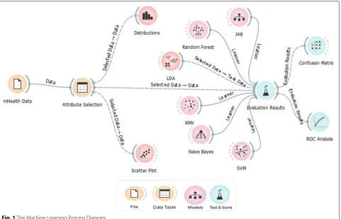
Figure1 illustrates the high-level machine learning pro-cess diagram used in the paper. The study explored the probable predictors of diabetes hospital re-admission among the hospitals using machine learning techniques along with other exploratory methods. The dataset con-sists of 55 attributes and only 18 were used as per the scope of the study. The performance of the models is eval-uated using the conventional confusion matrix and ROC efficiency analysis. The final re-admission model is based on the best performing model as per the true positive rates, sensitivity and specificity.
Linear discriminant analysis
Fig. 1The Machine Learning Process Diagram
of the class that it creates using the conventional statistical techniques.
μ= 1 nk
(x) (1)
Whereμis the mean of each input attribute (x) for each class (k) andnis the total number of observations in the dataset. The variance associated with the classes is also computed using the following conventional method.
σ2= 1
n−k
(x−μ)2 (2)
In Eq.2, sigma squared is the variance across all instance serving as input in the model,kis the number of classes, andn is the number of observations or instance in the dataset.μis the mean and is computed using Eq.1.
Besides the assumptions, the algorithm makes predic-tion using a probabilistic approach that can be summa-rized in two steps. Firstly, LDA classifies predictors and assigns them to a class based on the value of the posterior probability denoted as
π y=ix
(3)
The objective is to minimize the total probability of mis-classifying the features, and this approach relies on Bayes’
rule and the Gaussian distribution assumption for class means where:
π xy = i
(4)
Secondly, LDA finds a linear combination of the predic-tors that return the optimum predictor value, and this study uses the latter. LDA algorithm can be implemented in five basic steps. First, in performing LDA classification, the d-dimensional mean vectors are computed for the classes identified in the dataset using the mean approach (Eq.1). The variance and the normality assumption must be checked before proceeding. Second, both within and between-class scatters are computed and returned as a matrix. The within-class scatter or distances are com-puted based on Eq.5.
Swithin=
c
i=1
Si (5)
and
Si = n
x∈Di
where i is the scatter for every class identified in the dataset andμis the mean of the classes computed using Eq.1.
The Between-class scatter is calculated using Eq.7.
Sbetween = c
i−1
Ni(μi − μ ) (μi − μ)T (7)
In Eq. 7, S is general mean value whileμ andN refers to the sample mean and sizes of identified classes respec-tively. The third step involves solving Eigenvectors asso-ciated with the product of the within-class and out-class matrices. The fourth step involves sorting the linear dis-criminant to identify the new feature subspace. The selec-tion and sorting using decreasing magnitudes of Eigen-values. The last step involves the transformation of the samples or observations onto the new linear discrimi-nant sub-spaces. The pseudo-code for LDA is presented in Algortihm 1.
Algorithm 1Linear Discriminant Analysis
1:
D=xTi ,yi
n i=1 : 2: Di=
xTj |yi=ci,j=1, ...,n
,i=1, 2 //declaration of class-specific subsets 3: μi=mean(Di),i=1, 2
//calculation of class means 4: B=(μ1−μ2) (μ1−μ2)T
//Computation of between-class scatter 5: Zi=Di−1niμTi ,i=1, 2
// Center scatter matrix 6: Si=ZiTZi,i=1, 2
//The scatter of the respective classes 7: S=S1+S2
//Computation of within-class scatter distances 8: λ1,w=eigen
S−1B
//Computation of eigenvector using dominance
For the classes i, the algorithm divides the data into
D1 and D2 then calculates the within and between the class distances, and the best linear discriminant is a vec-tor obtained from the product of transpose of within-class and between-class scatter matrices.
Random forest
Random forest is a variant of decision degree growing technique and it is different from the other classifiers, because it supports random growth branches within the selected subspace. The random forest model predicts the outcome based on a set of random base regression trees. The algorithm selects a node at each random base regression and split it to grow the other branches. It
is important to note that Random Forest is an ensem-ble algorithm because it combines different trees. Ide-ally, ensemble algorithms combine one or more classifiers with the different types. Random forest can be thought of a bootstrapping approach for improving the results obtained from the decision tree. The algorithm works in the following order. First, it selects a bootstrap sam-pleS(i)from the sample space and the argument denoting the bootstrap sample refers to the ith bootstrap. The algorithm learns a conventional decision tree although through implementation of a modified decision tree algo-rithm. The modification is specific and is systematically implemented as the tree grows. That is, at each node of decision tree, instead of implementing an iteration for all possible feature split, RF randomly selects a subset of features such that f ⊆ F and then splits the fea-tures in the subset (f). The splitting is based on the best feature in the subset and during implementation, the algorithm chooses the subset that it is much smaller than the set of all features. Small size of subset reduces the burden to decide on the number of features to split since datasets with large size subsets tend to increase the computational complexity. Hence, the narrowing of the attributes to be learned improves the learning speed of the algorithm.
Algorithm 2Random Forest (Decision Tree Ensemble) Prerequisite: Specify the training set S := (x1,y1), ...,(xn,yn) the set of all features F, and the
number of trees to be included in the forestB 1: function RANDOM FOREST(S,F)
2: H←0
3: for i∈1, ...,Bdo
4: S(i)←1 Bootstrap sample drawn fromS 5: hi RandomizedTreelearn(S(i), F)
6: H←H∪ {hi}
7: end for 8: returnH 9: end function
10: function RANDOMIZEDTREELEARN(S,F) 11: At each node:
12: f ←Draw a small subset ofF 13: Split the best feature inf
14: return The Learned Tree (Model) 15: end function
The algorithm uses bagging to implement the ensem-ble decision tree, and it is prudent to note that bagging reduces the variance of the decision tree algorithm.
Support vector machine
analysis. One of the variables in the training sample should be categorical so that the learning process assigns new categorical value as part of the predictive outcome. As such, SVM is a non-likelihood binary classifier lever-aging the linear properties. Besides classification and regression, SVM detects outliers and is versatile when applied to dimensionality high [1]. Ideally, a training vec-tor variable, that has at least two categories, is defined as follows:
xi∈Rp,i=1, ...,n (8)
wherexirepresents the training observation andRp
indi-cates the real-valued p-dimensional feature space and predictor vector space. A pseudo-code for a simple SVM algorithm is illustrated:
Algorithm 3Support Vector Machine)
AttributeSupportVector(ASV)
={Closest Attribute Pair from Opposite Classes} 1: while margin constraint violating points exist do 2: Find the violator
3: ASV = ASV∪Violator
4: if anyαp<0 because of addition of c to S then
5: ASV= ASVp
6: Repeat all the violating points are pruned 7: end if
8: end while
The algorithm searches for candidate support vectors denoted asSand it assumes thatSV occupies as a space where the parameters of the linear features of the hyper-plane are stored.
k-nearest neighbor
kNN classifies data using the same distance measure-ment techniques as LDA and other regression-based algo-rithms. In classification application, the algorithm pro-duces class members while in regression application it returns the value of a feature or a predictor [9]. The technique can identify the most significant predictor and as such was given preference in the analysis. Nonethe-less, the algorithm requires high memory and is sensi-tive to non-contributed features despite being considered insensitive to outliers and versatile among many other qualifying features. The algorithm creates classes or clus-ters based on the mean distance between data-points. The mean distance is calculated using the following equation.
(x)= 1 k.
(xi,yi)∈kNN(x,L,K)yi (9)
In Eq.9,kNN(x,L,K),kdenotes theKnearest neigh-bors of the input attribute (x) in the learning set space (i).
The classification and prediction application of the algo-rithm depends on the dominantkclass and the predictive equation is as the following:
(x)=argmaxc∈y.(xi,yi)∈N(x,L,K)yi (10)
It is imperative to note that output class consists of members from the target attribute and the distance used in assigning the attributes to classes is based on Euclidean distance. The implementation of the algorithm consists of six steps. The first step involves the computation of Euclidean distance. In the second step, the computed n distances are arranged in a non-decreasing order, and in the third step, a positive integerkis drawn from the sorted Euclidean distances. In the fourth step, k-points corre-sponding to the k-distances are established and assigned based on proximity to the center of the class. Finally, for
k >0 and for (number of points in the i, an attribute x
is assigned to that class ifki > kj for all i = jis true.
Algorithm 4 shows the kNN steps process:
Algorithm 4k-Nearest Neighbor)
Preconditions: Specify training data (X), class labels (Y), and unknown sample (x)
1: Classify (X,Y,x) 2: fori=1 tomdo
3: Compute distanced(Xi,x)
4: end
5: for Compute Set I contains the minimum sets of k
distancesd(Xi,x)
6: Return majority label for{Yi;i∈I}
Naïve Bayes
Even though Naïve Bayes is one of the supervised learning techniques, it is probabilistic in nature so that the classifi-cation is based on Naïve Bayes’ rules of probability, espe-cially those of association. Conditional probability is the construct of Naïve Bayes classifier [9–16]. The algorithm assigns instance probabilities to the predictors parsed in a vector format representing each probable outcome. Naïve Bayes classifier is the posterior probability that the divi-dend of the product of prior with likelihood and evidence returns. The construction of the model from the output of the analysis is quite complex although the probabilistic computation from the generated classes is straightforward [17–22]. The Bayes Theorem upon which the Naïve Bayes classifier is based can be written as follows:
P(μ|ν)= P(ν|μ)P(μ)
P(ν) (11)
vis the basis of Naïve Bayes classifier. The classifier uses maximum likelihood hypothesis to assign data points to classes. The algorithm assumes that each feature is inde-pendent and makes equal contribution to the outcome or all features belonging to the same class have the same influence on that class. In Eq. 11, the algorithm com-putes the probability of event μprovided thatvalready occurred, and as such vis the evidence and the proba-bilityP(μ)is regarded as the priori probability. That is, it refers to probability obtained before seeing the evi-dence while the conditional probabilityP(μ|ν) is priori probability of vsince it is a probability computed with evidence.
J48
J48 is one of the decision tree growing algorithm. How-ever, J48 is the reincarnation of the C4.5 algorithm, which is an extension of the ID3 algorithm [23]. As such, J48 is a hierarchical tree learning technique and it has several mandatory parameters including the confidence value and the minimum learning instance, which are translated to branches and nodes in the final decision tree [23–29]. Data assembly and pre-processing
The study used diabetes data that was collected across 130 hospitals in the US in the years between 1999–2008 [30]. The dataset includes data systematically composed from contributing electronic health records’ providers that contained encounter data such as inpatient, outpa-tient and emergency, demographics, provider specialty, diagnosis, in-hospital procedures, in-hospital mortality, laboratory and pharmacy data. The complete list of the features and description is provided in Table S1
(Additional file 1). The data has 55 attributes, about 100,000 observations, and has missing values. However, the study used a sample based on the treatment of dia-betes. In specific, of the 100,000 cases, 78,363 meet the inclusion criteria since they received medication for diabetes. Consequently, the study explored re-admission incidences among patients who had received treatment. The amount of missing information, the type of the data (categorical or numeric) that guided the data clean-ing process, re-admission, Insulin prescription, HbA1c test results, and observed changes were retained as the major out-come associated with time spent in the hospi-tal, the number of diagnoses, lab procedures, procedures, and medications [31, 32]. Of the 55, only 18 variables were selected as per the scope for analysis and even about 8 of the selected served as proxy controls. The study was split into 70% training and 30% validation subsets.
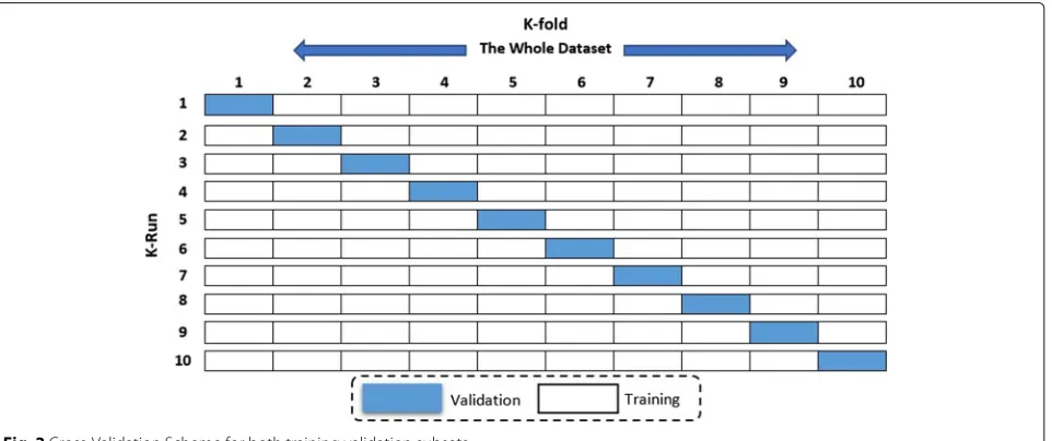
K-fold validation
To improve the overall accuracy and validate a model, we relied on the 10-fold cross validation method applied for estimating accuracy. The training dataset is split into k-subsets and the subset held out while the model is fully trained on remaining subsets. Figure2illustrates the val-idation method. The K-fold Cross-valval-idation method uti-lizes the defined training feature set and randomly splits it into k equal subsets. The model is trained k times. During each iteration, 1 subset is excluded for use as validation. This technique reduces over-fitting issues, which occurs when a model trains the data too closely to a set of data, which can result in failure to predict future information reliably [2,12,33].
Discussion
Exploratory analysis
Of the 47.7% diabetic patients who were readmitted, 11.6% stayed in the hospital for less than 30 days while 36.1% stayed for more than 30 days. A majority (52.3%) of those who stayed for more than 30 days did not receive any medical procedures during the first visit. In general, diabetic patients who received a fewer num-ber of lab procedures, treatment procedures, medica-tions, and diagnoses are more likely to be readmitted than their counterparts. Furthermore, the more frequent a patient is admitted as an in-patient the less likely the probability of re-admission. Our study indicated that, women (53.3%) and Caucasian (74.6%) diabetic patients are more vulnerable to re-admission than male and the other races. Besides several lab procedures, medica-tions, and diagnoses, insulin administration and HbA1c results exacerbate the re-admission rates among diabetic patients.
Scatterplots
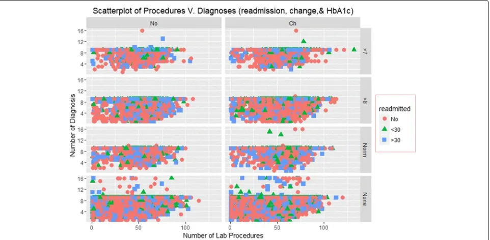
The Scatterplots of re-admission incidences with an over-lay of HbA1c measurements and change recorded at the time of discharge are shown in Figs.3and4.
Figure 3 illustrates the Scatterplot of the number of diagnoses and lab procedures that patient received for re-admission rates. The figures have 8 panels display-ing scatters of diagnoses and lab procedures for differ-ent instances of HbA1c results and change. The plot shows that patients who had negative HbA1c tests results received several diagnosis and very few were readmitted.
Those who received less than 10 diagnoses and less than 70 procedures were more likely to be readmitted. None of the patients received more than diagnosis and a majority were admitted for more than 30 days.
Figure4depicts a scatter plot of a number of diagnoses and lab procedures. The re-admission rates are quite dif-ferent between a group of patients who noted change at discharge than those who did not. Those who failed to note significant improvement at discharge received more than 50 medications and less than 10 diagnoses. However, re-admission is higher among those who noted improve-ment at discharge.
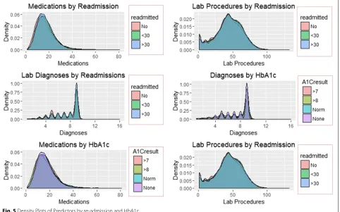
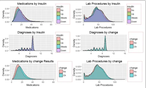
Density distributions
The distribution of re-admission and subsequent patterns associated with reported change and results of HbA1c are shown in Figs.5and6.
Figures 5 and 6 illustrate the density distribution of number of medications, lab procedures, and diagnoses grouped by re-admission, HbA1c results, insulin admin-istration change at discharge. Notably, the distribution density of the number of lab procedures, medications, and diagnoses are the same for grouping categories. Figure6 shows significant differences in the number of medications and lab procedures. For instance, the aver-age number of medications differs between ’No’, ’Up’, ’Steady’, and ’Down’ insulin categories. A similar differ-ence in mean of the number of medications is observed in the change distribution curve with those recording change at discharge receiving more medications than their counterparts.
Fig. 4Scatterplot of Medications and Diagnoses
Fig. 6Density Plots of Predictors by Insulin and change
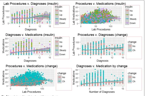
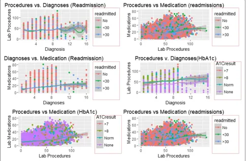
Smooth linear fits
Figures 7 and 8 illustrate the smooth line fits asso-ciated with Scatterplots. The smoothen fits include a 95% confidence interval and demonstrates the likely performance of linear regression models in forecasting re-admission.
Figures7and8depict smooth linear fits of the Scatter-plots and density Scatter-plots in Figs.3,4,5, and6. The figures illustrate that the number of lab procedures has linear relationships with the number of diagnoses although the data is likely to be heteroskedastic. The number of diag-noses and medications also have the same relationship and plot patterns. For medication versus procedures, the rela-tionship is linear and change in diabetes status increases with medications and lab procedures. As for re-admission, incidents of more than 30 days re-admission reduced with increasing number of diagnoses, lab procedures, and med-ications. Similarly, the probability of detecting HbA1c increases with increasing number of diagnoses and lab procedures.
Model evaluation
The performance of the models in predicting re-admission incidence was based on the confusion matrix and in specific the percentage of the correctly predicted read-mission categories.
Table 1 depicts that Naïve Bayes correctly classified the admission rates less than 30 days and none re-admission incidences. SVM accurately classified 48.3% of the re-admission incidence exceeding 30 days. The objec-tive is to obtain the performing model.
Individual model performance
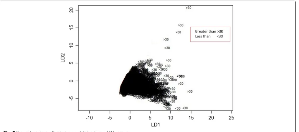
The LDA model yields two linear discriminants LD1 and LD2 with proportion trace of 0.9646 and 0.0354 respec-tively. Hence, the first LD explains more than 96.46% of the between-group variance while the second account for 3.54% of the between-group variance.
LD1=003∗ Lab Procedures −0.102∗Procedures +0.08∗ Medications+0.18∗ Emergency +0.67 Inpatient
+0.17Diagnoses (12)
Figure9illustrates the plot of LD1 versus LD2. Equation 12 depicts the profile of diabetic patients.
Fig. 7Smooth Linear Fits with Insulin and Change as Facets
lab procedures, diagnoses, and medications. However, the rates are higher among patients who tested positive for HbA1c and did not fail to receive insulin treatment (Fig.3).
SVM classified the readmitted diabetic patients into three classes using a polynomial of degree 3 suggest-ing that diabetes re-admission cases do not have a lin-ear relationship with the predictors. As an inference, the polynomial relationship illustrated by the kernel and degree of the SVM indicates higher re-admission rates among patients discharged without any significant changes (Fig.4). Naïve Bayes classifier yields two classes using the Laplace approach. The classification from the model depicts a reduced likelihood of re-admission in cases where the patients undergo a series of laboratory tests, rigorous diagnosis, proper medication, and dis-charge after confirmation of improvement. The density distributions in Figs. 5 and 6 compliments the findings of the model. In specific, the distributions of the num-ber of medications and lab procedures show a noticeable difference in the distribution when considering insulin administration as part of treatment. Regarding aggrega-tion of the distribuaggrega-tion of the number of medicaaggrega-tions and lab procedures by status at discharge (change), the
Fig. 8Smooth Linear Fits with re-admission and HbA1c as Facets
several diagnoses improve health outcomes and reduce re-admission.
Best fit model
The best fitting model is based on the performance mea-sures summarized in Table 2. The key decision relies on the efficiency of the model in predicting the re-admission rates and the area under the curve (AUC) and precision/recall curve are the best measures for such a task.
Table2illustrates that Naïve Bayes is the most sensitive and efficient model for learning, classifying and predicting re-admission rates using mHealth data. It has an efficiency
Table 1True Positive Rate Comparison Table
Model <30 days >30 days No
Random Forest 21.0% 42.8% 60.5%
kNN 17.8% 40.3% 59.6%
Naïve Bayes 23.6% 46.6% 61.2%
SVM 12.2% 48.3% 55.9%
J48 17.3% 40.4% 60.3%
of 64% and a sensitivity of 52.4%. The ROC curves asso-ciated with the predictions of re-admission that exceeded 30 days are displayed in the figures below.
The larger the area covered the more efficient the model is, and this principle Fig.10depicts that Naïve Bayes is the most efficient.
Naïve bayes analysis
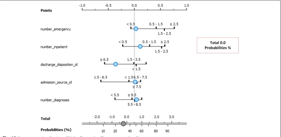
The model focused on the top 5 best factors (exposures) that contributed to re-admission for less and more than 30 days. The association between the exposures and outcome (re-admission instances) are given as log odds ratio in the nomograms illustrated in Fig.11. The three classes model are Class 0 (No re-admission), Class 1 (re-admission for less than 30 days), and Class 3 (re-admission for more than 30 days).
Fig. 9Plot of two linear discriminants obtained from LDA learner
Figure 12 depicts the exposure factors with absolute importance on Class 1 including the number of emer-gencies, the number of patients, discharge disposition ID, time in hospital ID, and number of diagnoses. The log odds ratios display the association between these exposure factors to lack of re-admission after discharge. The conditional probability for re-admission after dis-charge based on these exposure factors is 14%. In specific, there is a 48% chance of re-admission for patients with a number of diagnoses between 8.5 and 9.5, and a 52% chance for those with diagnoses between 5.5 and 8.5. Similarly, those spending between 2.5 to 3.5 days in the hospital is more likely to be readmitted (59%) for less than 30 days than their counterparts with 41% chance of re-admission. Finally, those with fewer emergency admission history stand higher chances of re-admission (80%) than those with sufficient emergency admission history.
Figure 13 depicts the exposure factors with absolute importance on Class 2 including the number of emer-gencies, the number of patients, discharge disposition ID, admission source ID, and number of diagnoses. The log
Table 2Comparison of model efficiency and sensitivity
Model AUC CA F1 Precision Recall
kNN 0.575 0.499 0.489 0.482 0.499
J48 0.578 0.490 0.487 0.485 0.490
SVM 0.547 0.475 0.421 0.483 0.475
Random Forest 0.602 0.529 0.509 0.499 0.529
Naïve Bayes 0.640 0.566 0.524 0.519 0.566
odds ratios illustrate the association between these expo-sure factors to lack of re-admission after discharge. The conditional probability for re-admission after discharge based on these exposure factors is 0.42. The number of emergency admission increases re-admission chances by 80% for those with least history. Further, those with higher inpatient admission history have 65% chance of re-admission for more than 30 days. Most importantly, patients who undergo more than 9.5 diagnoses tests have 70% chance of re-admission for more than 30 days after discharge.
Conclusion
Fig. 10ROC curves illustrating the Areas Under Curve for the models
Fig. 12Nomogram visualization of Naïve Bayes classifier on target class 1
emphasis on the importance of emergency admission and in-patient treatment on re-admission rates. kNN models lead to the conclusion that fewer number of lab pro-cedures, diagnoses, and medications lead to increased higher re-admission rates. Diabetic patients who do not
undergo vigorous lab assessments, diagnosis, medica-tions are more likely to be readmitted when discharged without improvements and without receiving insulin administration, especially if they are women, Caucasians, or both.
Supplementary information
Supplementary informationaccompanies this paper at https://doi.org/10.1186/s12911-019-0990-x.
Additional file 1:List of features and descriptions in the experiment datasets.
Abbreviations
AI: Artificial intelligence; ANOVA: Analysis of variance; C4.5: Data mining algorithm; DA: Discriminant analysis; HbA1c: Glycated hemoglobin test; ID3: Iterative dichotomiser 3; J48: Decision tree J48; KNN: K-nearest neighbors; LA: Linear discriminant; ML: Machine learning; NB: Naive Bayes; Non-ICU: Non intensive care unit; RF: Random forest; ROC: Receiver operating characteristic; SVM: Support vector machine
Acknowledgments
The data sources used in the paper was retrieved from UCI Machine Learning Repository as submitted by the Center for Clinical and Translational Research. The organization and the characteristics of the data made it easy to complete classification and clustering tasks. We are also grateful to the artificial intelligence department for providing the necessary support to carry out such a research.
About this supplement
This article has been published as part ofBMC Medical Informatics and Decision Making Volume 19 Supplement 9, 2019: Proceedings of the 2018 International Conference on Intelligent Computing (ICIC 2018) and Intelligent Computing and Biomedical Informatics (ICBI) 2018 conference: medical informatics and decision making. The full contents of the supplement are available online athttps:// bmcmedinformdecismak.biomedcentral.com/articles/supplements/volume-19-supplement-9.
Authors’ contributions
All authors read and approved the final manuscript.
Author details
1The Artificial Intelligence Department-, Dubai, UAE.2Liverpool John Moores University, Liverpool, UAE.3The University of Anbar, Al-Tameem Street, 55431 Al-Anbar, Al-Ramadi, Iraq.4Kazan Federal University, Kremlyovskaya St, 420008 Kazan, Republic of Tatarstan, Russia.5Department of Computer Science, Al-Maarif University College, Anbar, 31001 The city of Ramadi, Iraq.
Published: 12 December 2019
References
1. Guoa W-L, DS H. An efficient method to transcription factor binding sites imputation via simultaneous completion of multiple matrices with positional consistency. Mol BioSyst. 2017;13(9):1827–37.https://doi.org/ 10.1039/C7MB00155J.
2. Strack B, DeShazo JP, Clore JN. Impact of hba1c measurement on hospital readmission rates: Analysis of 70,000 clinical database patient records. BioMed Res Int. 2014;11:.https://doi.org/10.1155/2014/781670. 3. Bengio Y, Grandvalet Y. No unbiased estimator of the variance of k-fold
cross-validation. J Mach Learn Res. 2004;5:1089–105.
4. Bo LJ. Song: Naive bayesian classifier based on genetic simulated annealing algorithm. Procedia Eng. 2011;23:504–9.https://doi.org/10. 1016/j.proeng.2011.11.2538.
5. Chan M. Global report on diabetes. Report. 2016;978:9241565257.https:// apps.who.int/iris/bitstream/handle/10665/204871/9789241565257_eng %.pdf;jsessionid=BE557465C4C16EF288D80B9E41AE01C8?sequence=1. 6. Chen Peng LZ, Huang D-s. Discovery of relationships between long
non-coding rnas and genes in human diseases based on tensor completion. IEEE Access. 2018;6:59152–62.https://doi.org/10.1109/ ACCESS.2018.2873013.
7. Bansal D, Khanna K, Chhikara R, Gupta P. Comparative analysis of various machine learning algorithms for detecting dementia. Procedia Comput Sci. 2018;132:1497–502.https://doi.org/10.1016/j.procs.2018.05.102. 8. Deepti Sisodia DSS. Prediction of diabetes using classification algorithms.
Procedia Comput Sci. 2018;132:1578–85.https://doi.org/10.1016/j.procs. 2018.05.122.
9. Kavakiotis I, Tsave O, Salifoglou A, Maglaveras N, Vlahavas I, Chouvarda I. Machine learning and data mining methods in diabetes research. Comput Struct Biotechnol J. 2017;15:104–16.https://doi.org/10.1016/j. csbj.2016.12.005.
10. Chuai G, Jifang Y, Chen M, et al. Deepcrispr: optimized crispr guide rna design by deep learning. Genome Biol. 2018;19(1):18.
11. Yi H-C, Huang D-S, Li X, Jiang T-H, Li L-P. A deep learning framework for robust and accurate prediction of ncrna-protein interactions using evolutionary information. Mol Ther-Nucleic Acids. 2018;1(11):337–44. https://doi.org/10.1016/j.omtn.2018.03.001.
12. Ling H, Kang W, Liang C, Chen H. Combination of support vector machine and k-fold cross validation to predict compressive strength of concrete in marine environment. Constr Build Mater. 2019;206:355–63. https://doi.org/10.1016/j.conbuildmat.2019.02.071.
13. Harleen Kaur VK. Predictive modelling and analytics for diabetes using a machine learning approach. Appl Comput Inform. 2018.https://doi.org/ 10.1016/j.aci.2018.12.004.
14. Zhang H, Yu P, et al. Development of novel prediction model for drug-induced mitochondrial toxicity by using naïve bayes classifier method. Food Chem Toxicol. 2017;10:122–9.https://doi.org/10.1016/j.fct. 2017.10.021.
15. Donzé J, Bates DW, Schnipper JL. Causes and patterns of readmissions in patients with common comorbidities: retrospective cohort study. BMJ. 2013;347(7171):.https://doi.org/10.1136/bmj.f7171.
16. Smith DM, Giobbie-Hurder A, Weinberger M, Oddone EZ, Henderson WG, Asch DA, et al. Predicting non-elective hospital readmissions: a multi-site study. Department of veterans affairs cooperative study group on primary care and readmissions. J Clin Epidemiol. 2000;53(11):1113–8. 17. Han J, Choi Y, Lee C, et al. Expression and regulation of inhibitor of dna binding proteins id1, id2, id3, and id4 at the maternal-conceptus interface in pigs. Theriogenology. 2018;108:46–55.https://doi.org/10.1016/j. theriogenology.2017.11.029.
18. Jiang L, Wang D, Cai Z, Yan X. Survey of Improving Naive Bayes for Classification. In: Alhajj R, Gao H, et al., editors. Lecture Notes in Computer Science. Springer; 2007.https://doi.org/10.1007/978-3-540-73871-8_14. 19. Jianga L, Zhang L, Yu L, Wang D. Class-specific attribute weighted naive
bayes. Pattern Recogn. 2019;88:321–30.https://doi.org/10.1016/j.patcog. 2018.11.032.
20. Han Lu LW, Zhi S. An assertive reasoning method for emergency response management based on knowledge elements c4.5 decision tree. Expert Syst Appl. 2019;122:65–74.https://doi.org/10.1016/j.eswa.2018.12.042. 21. Skriver MVJKK, Sandbæk A, Støvring H. Relationship of hba1c variability,
absolute changes in hba1c, and all-cause mortality in type 2 diabetes: a danish population-based prospective observational study. Epidemiology. 2015;3(1):8.https://doi.org/10.1136/bmjdrc-2014-000060.
22. ADA: Economic Costs of Diabetes in the U.S. in 2012. Diabetes Care; 2013. 23. Sun NJDL, Sun B, Wu MY-C. Lossless pruned naive bayes for big data
classifications. Big Data Res. 2018;14:27–36.https://doi.org/10.1016/j.bdr. 2018.05.007.
24. Nima Shiri Harzevili SHA. Mixture of latent multinomial naive bayes classifier. Appl Soft Comput. 2018;69:516–27.https://doi.org/10.1016/j. asoc.2018.04.020.
25. Nongyao Nai-arun RM. Comparison of classifiers for the risk of diabetes prediction. Procedia Comput Sci. 2015;69:132–42.https://doi.org/10. 1016/j.procs.2015.10.014.
26. Arar OFKA. A feature dependent naive bayes approach and its application to the software defect prediction problem. Appl Soft Comput. 2017;59: 197–209.https://doi.org/10.1016/j.asoc.2017.05.043.
27. Wyckoff OPCCB, Ciarkowski SL. Gianchandani: The relationship between diabetes mellitus and 30-day readmission rates. Clin Diabetes Endocrinol. 2017;3(3):8.https://doi.org/10.1186/s40842-016-0040-x.
28. Ranjit Panigrahi SB. Rank allocation to j48 group of decision tree classifiers using binary and multiclass intrusion detection datasets. Procedia Comput Sci. 2018;132:323–32.https://doi.org/10.1016/j.procs.2018.05.186. 29. Dungan KM. The effect of diabetes on hospital readmissions. J Diabetes
Sci Technol. 1045;6(5):.
30. Sajida Perveen MSea. Performance analysis of data mining classification techniques to predict diabetes. Procedia Comput Sci. 2016;82:115–21. https://doi.org/10.1016/j.procs.2016.04.016.
32. Kripalani SAB, Theobald CN, EE V. Reducing hospital readmission rates: current strategies and future directions. Annu Rev Med. 2014;65:471–85. https://doi.org/10.1146/annurev-med-022613-090415.
33. Wong T-T. Parametric methods for comparing the performance of two classification algorithms evaluated by k-fold cross validation on multiple data sets. Pattern Recogn. 2017;65:97–107.https://doi.org/10.1016/j. patcog.2016.12.018.
34. Wang Xiaohu WL, Nianfeng L. An application of decision tree based on id3. Phys Procedia. 2012;25:1017–21.https://doi.org/10.1016/j.phpro. 2012.03.193.
35. Trishan Panch PS, Atun R. Artificial intelligence, machine learning and health systems. J Global Health. 2018;8(2):.https://doi.org/10.7189/jogh. 08.020303.
36. Wenzheng Bao ZJ, Huang D-S. Novel human microbe-disease association prediction using network consistency projection. BMC Bioinformatics. 2017;18(S116):173–259.https://doi.org/10.1186/s12859-017-1968-2. 37. Wu J. A generalized tree augmented naive bayes link prediction model. J
Comput Sci. 2018;27:206–17.https://doi.org/10.1016/j.jocs.2018.04.006. 38. Mu YFBHUZXea. Pan C: Efficacy and safety of linagliptin/metformin
single-pill combination as initial therapy in drug-naïve asian patients with type 2 diabetes. Diabetes Res Clin Pract. 2017;124:48–56.https://doi.org/ 10.1016/j.diabres.2016.11.026.
39. Zhen Shen WB, Huang D-S. Recurrent neural network for predicting transcription factor binding sites. 2018;8(15270):10.https://doi.org/10. 1038/s41598-018-33321-1.
Publisher’s Note