https://doi.org/10.5194/amt-11-1273-2018 © Author(s) 2018. This work is distributed under the Creative Commons Attribution 4.0 License.
Calibration and field testing of cavity ring-down laser spectrometers
measuring CH
4
, CO
2
, and
δ
13
CH
4
deployed on towers in the
Marcellus Shale region
Natasha L. Miles1, Douglas K. Martins1,a, Scott J. Richardson1, Christopher W. Rella2, Caleb Arata2,3, Thomas Lauvaux1, Kenneth J. Davis1, Zachary R. Barkley1, Kathryn McKain4, and Colm Sweeney4 1Department of Meteorology and Atmospheric Science, The Pennsylvania State University, University Park, Pennsylvania 16802, USA
2Picarro, Inc., Santa Clara, California 95054, USA
3Department of Environmental Science, Policy, and Management, University of California, Berkeley, California 94720, USA 4National Oceanic and Atmospheric Administration, University of Colorado, Boulder, Colorado 80305, USA
acurrent address: FLIR Systems, Inc., West Lafayette, Indiana 47906, USA Correspondence:Natasha L. Miles ([email protected])
Received: 3 October 2017 – Discussion started: 16 October 2017
Revised: 23 January 2018 – Accepted: 28 January 2018 – Published: 5 March 2018
Abstract. Four in situ cavity ring-down spectrometers (G2132-i, Picarro, Inc.) measuring methane dry mole frac-tion (CH4), carbon dioxide dry mole fraction (CO2), and the isotopic ratio of methane (δ13CH4) were deployed at four towers in the Marcellus Shale natural gas extraction region of Pennsylvania. In this paper, we describe laboratory and field calibration of the analyzers for tower-based applications and characterize their performance in the field for the period January–December 2016. Prior to deployment, each analyzer was tested using bottles with various isotopic ratios, from biogenic to thermogenic source values, which were diluted to varying degrees in zero air, and an initial calibration was performed. Furthermore, at each tower location, three field tanks were employed, from ambient to high mole fractions, with various isotopic ratios. Two of these tanks were used to adjust the calibration of the analyzers on a daily basis. We also corrected for the cross-interference from ethane on the isotopic ratio of methane. Using an independent field tank for evaluation, the standard deviation of 4 h means of the iso-topic ratio of methane difference from the known value was found to be 0.26 ‰δ13CH4. Following improvements in the field tank testing scheme, the standard deviation of 4 h means was 0.11 ‰, well within the target compatibility of 0.2 ‰. Round-robin style testing using tanks with near-ambient iso-topic ratios indicated mean errors of −0.14 to 0.03 ‰ for each of the analyzers. Flask to in situ comparisons showed
mean differences over the year of 0.02 and 0.08 ‰, for the east and south towers, respectively.
1 Introduction
uantification of regional greenhouse gas emissions resulting from natural gas extraction activities is critical for determi-nation of the climate effects of natural gas usage compared to coal or oil. Studies have shown that the emission rates as a percentage of production vary significantly from reservoir to reservoir. An aircraft-based mass balance study in the Uin-tah basin in UUin-tah (Karion et al., 2013; Rella et al., 2015) found a methane emission rate of 6.2–11.7 % of production, exceeding the 3.2 % threshold for natural gas climate bene-fits compared to coal determined by Alvarez et al. (2012). In the Denver–Julesburg basin in Colorado, Pétron et al. (2014) found an emissions rate of 4 % of production, again using an aircraft mass balance approach. The Barnett Shale, one of the largest production basins in the United States with 8 % of total US natural gas production, was found to exhibit a lower emission rate of 1.3–1.9 % (Karion et al., 2015). Using a model optimization approach for aircraft data, Barkley et al. (2017) found the weighted mean emission rate from un-conventional natural gas production and gathering facilities in the Marcellus region in northeastern Pennsylvania, a re-gion with mostly dry natural gas, to be only 0.36 % of total gas production.
Aircraft-based studies cover large areas, but the temporal coverage is limited. Tower-based networks offer a comple-mentary approach, making continuous measurements over long periods of time. At the Boulder Atmospheric Observa-tory (BAO) tall tower, daily flask measurements are found to contain enhanced levels of methane and other alkanes, compared to the other tall towers in the National Oceanic and Atmospheric Administration (NOAA) network (Pétron et al., 2012). Tower measurements allow for continuous mea-surements in the well-mixed boundary layer which are influ-enced by both nearby sources and the integrated effect of the upstream emissions. While towers provide near-continuous coverage of regional emissions, specific emissions sources with specific isotopic signatures are often diluted by mixing, making the differences from background very small.
Differentiating CH4emissions from natural gas activities from other sources (e.g., wetlands, cattle, landfills) is key to documenting the greenhouse gas impact of natural gas pro-duction and to evaluating the effectiveness of emissions re-duction activities. The isotopic ratio of methane (δ13CH4) is particularly useful in this regard (Coleman et al., 1995). In general, heavy isotope ratios are characteristic of thermo-genic CH4sources (i.e., fossil-fuel-based), and light isotope ratios are characteristic of biogenic sources (Dlugokencky et al., 2011). Schwietzke et al. (2016) compiled a comprehen-sive database of isotopic methane source signatures, indicat-ing signatures of−44.0 ‰ for globally averaged fossil-fuel sources of methane;−62.2 ‰ for globally averaged micro-bial sources such as wetlands, ruminants, and landfills; and
−22.2 ‰ for globally averaged biomass burning sources. At-mospheric measurements ofδ13CH4have been used to
parti-tion emissions of CH4into source categories (e.g., Mikaloff Fletcher et al., 2004a, b; Kai et al., 2011). It is important to note, however, that, for fossil-fuel sources of methane, isotopic ratios of methane vary significantly from reservoir to reservoir (e.g., Townsend-Small et al., 2015; Rella et al., 2015), and with depth in a single reservoir (Molofsky et al., 2011; Baldassare et al., 2014).
The isotopic ratio of methane has traditionally been measured in the laboratory with continuous-flow gas chromatography–isotope ratio mass spectrometry, with re-peatability of±0.05 ‰ (Fisher et al., 2006). Röckmann et al. (2016) recently compared continuous in situ measure-ments of methane isotopic ratio using a dual isotope mass spectrometric system (IRMS) and a quantum cascade laser absorption spectroscopy (QCLAS)-based technique at the Cabauw tower site in the Netherlands. They showed that high-temporal-resolution methane isotopic ratio data can be used in conjunction with a global and a mesoscale model to evaluate CH4emission inventories. Röckmann et al. (2016) also used a moving Keeling plot approach to identify source isotopic ratios.
Cavity ring-down spectroscopy (CRDS) is another tech-nique for measurement of continuous in situ isotopic ratio of methane (Rella et al., 2015). CRDS is a laser-based tech-nique in which the infrared absorption loss caused by a gas in the sample cell is measured to quantify the mole frac-tion of the gas. The analyzers utilize three highly reflec-tive mirrors such that the flow cell has an effecreflec-tive optical path length of 15–20 km, allowing highly precise measure-ments. The temperature and pressure of the sample cell are tightly controlled, improving the stability of the measure-ments (Crosson, 2008). Rella et al. (2015) documented the operation of CRDS (Picarro, Inc., model G2132-i) analyz-ers, including cross-interference from other gases, and gen-eral calibration approach.
Furthermore, Rella et al. (2015) described the use of two tanks to correct for analyzer drift of the isotopic ratio mea-sured by the G2132-i analyzers. In this approach, the vari-ables of interest, i.e., the total methane mole fraction and the isotopic ratio, are directly calibrated. The drift terms in the calibration equations have differing dependence on mole fraction, requiring the use of at least two tanks for calibra-tion. For this study, three field tanks were deployed at each tower location, two for the field calibration and one as an independent test.
analyzers, field calibration approach, and calibration results. We determine the compatibility achieved for the isotopic measurements in the current field deployment, using an in-dependent field tank, round-robin style testing, and compar-isons to flasks as our primary metrics. We also evaluate the performance of the G2132-i analyzers in terms of CH4and CO2mole fractions measurements by comparing to a G2301 analyzer. We then describe the tower locations and compare differences in CH4mole fraction and isotopic ratio observed at the towers and use a Keeling plot approach to determine source isotopic signatures. Finally, we describe recommen-dations for future isotopic methane CRDS tower-based net-works.
2 Compatibility goals
Because this is the first network of multiple methane isotopic ratio continuous analyzers to date, the needed compatibility has not yet been defined. Thus, our compatibility goals for CO2and CH4mole fractions follow the WMO compatibility recommendation for global studies: 0.1 ppm for CO2(in the Northern Hemisphere) and 2 ppb for CH4(GAW Report No. 229, 2016). Here we use the term compatibility, as advised in the GAW Report No. 229 (2016), to describe the difference between two measurements, rather than the absolute accu-racy of those measurements.
For δ13CH4, we set our target compatibility at 0.2 ‰,
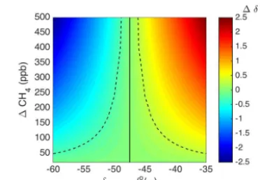
thought to be a reasonable goal based on laboratory test-ing prior to deployment and the results shown in Rella et al. (2015). This goal corresponds to the WMO extended com-patibility goal for the isotopic ratio of methane, which was deemed sufficient for regionally focused studies with large local fluxes. The measured signal at the towers is a mixture of the source and the background (Pataki et al., 2003), and the ability to distinguish between a biogenic and thermogenic source depends on the difference of the source isotopic sig-nature from background and the peak strength in terms of methane mole fraction. Equating the slope of a source and the background with the slope of a mixture and the background on a Keeling plot (Keeling, 1961), the measured isotopic ra-tio difference (1δ)is given by
1δ= δsource−δbackground
1CH4 CH4, measured
, (1)
where δsource and δbackground are the isotopic ratios of the source and the background, CH4, measured is the measured methane mole fraction, and1CH4is the difference between the measured mole fraction and the background. This equa-tion is represented graphically in Fig. 1. If there are two pos-sible sources in a region, a biogenic source at −60 ‰ and a thermogenic source at−35 ‰, for example, the difference in isotopic ratio difference is at least 3 times the compat-ibility goal of 0.2 ‰ (and thus distinguishable) for a peak strength of 50 ppb CH4or greater, assuming a measured CH4
Figure 1.Isotopic ratio difference from background (1δ)resulting from a mixture of background and source signatures, as a function of source isotopic ratio (δsource)and CH4mole fraction enhance-ment above background (1CH4). Here the source end-members are
−60 and−35 ‰. Background CH4mole fraction was assumed to be 2000 ppb, and background isotopic ratio−47.5 ‰ (vertical solid line). Dashed lines indicate−0.3 and 0.3 ‰ difference from back-ground.
mole fraction of 2000 ppb and a background isotopic ratio of
−47.5 ‰. In this case, the biogenic source would measure 0.3 ‰ above the background, as opposed to the thermogenic source measuring 0.3 ‰ below the background. As shown in Fig. 1, sources closer to the background in isotopic ratio require a larger peak in CH4and those further from the back-ground can be attributed with a smaller peak in CH4.
3 Allan standard deviation testing
Allan standard deviation testing (Allan, 1966) is a useful tool for testing the noise and drift response of instrumentation. The Allan standard deviation for each averaging interval is proportional to the range of values for each averaging inter-val. This range typically decreases for increasing averaging interval, as the noise is reduced through averaging. As the av-eraging interval increases, however, analyzer drift may con-tribute, placing an upper bound on the optimal averaging in-terval. Thus, the Allan deviation results are critical for defin-ing the minimum averagdefin-ing time required for a given target compatibility.
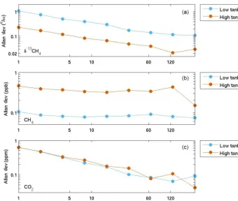
Figure 2.Allan standard deviation for(a)δ13CH4,(b)CH4, and(c)CO2for a high CH4mole fraction tank (9.7 ppm CH4,∼400 ppm CO2,
−38.3 ‰δ13CH4; orange) and a low (1.9 ppm CH4,∼400 ppm CO2,−23.7 ‰δ13CH4)tank (blue). Thexaxis is truncated to focus on minimum averaging times required to achieve the desired compatibility goals.
The resulting Allan standard deviations forδ13CH4, CH4, and CO2 are shown in Fig. 2. For the high tank, the Allan deviation forδ13CH4(Fig. 2a) was < 0.2 ‰ (our target com-patibility) for an averaging interval of 2 min (the averaging interval used each field calibration cycle of the high tank). To reduce the noise to < 0.1 ‰, an averaging interval of 4 min is sufficient (in addition to the time required for the transi-tion between gases). For the low tank, in order for the Al-lan standard deviation to be < 0.2 ‰, 32 min was required, and 64 min for 0.1 ‰ noise. Note that for much of the de-ployment the near-ambient mole fraction target tank was not sampled sufficiently within each day for the desired compat-ibility goals.
For CH4 (Fig. 2b), both the high- and low-tank Allan deviation were < 1 ppb for even a 1 min averaging inter-val. The CO2 levels in the high and low tanks were simi-lar (∼400 ppm), and an averaging interval of 6 min corre-sponded to Allan standard deviations of 0.3 ppm, and 64 min was necessary for 0.1 ppm (Fig. 2c). The performance of the G2132-i analyzers in terms of CO2 precision is worse than that of the G2301/G2401 analyzers primarily because a weaker spectral line is used (Rella et al., 2015).
4 Laboratory calibration
4.1 Experimental setup
Prior to field deployment, each analyzer was calibrated for CH4and CO2mole fraction. Four NOAA-calibrated tertiary standards (traceable to the WMO X2004 scale for CH4 and the WMO X2007 scale for CO2) were used for the lin-ear mole fraction calibration, as described in Richardson et al. (2017). These NOAA tertiary standards ranged between 1790 and 2350 ppb CH4, and between 360 and 450 ppm CO2. To calibrate the δ13CH4 measurement prior to deploy-ment, four different target mixing ratios, each at four dif-ferent known isotopic ratios, were tested by the four ana-lyzers using the experimental setup in Fig. 3. Commercially available isotopic standard bottles (Isometric Instruments, Inc., product numbers L-iso1, B-iso1, T-iso1, and H-iso1) were diluted with zero air to produce mixtures with vary-ing CH4mixing ratios andδ13CH4. The gravimetrically de-termined zero air (Scott Marrin, Inc.) was natural ultra-pure air, containing no methane or other alkanes but ambient lev-els of CO2. The isotopic calibration standard bottles each contained approximately 2500 ppm of CH4at−23.9,−38.3,
CRDS
CRDS
CRDS
CRDS Pump
Pump
Pump
Pump Mixing
volume 0.005–1 sccm
range MFC
1–200 sccm range MFC
Zero air (Scott-Marrin) 2500 ppm CH4
δ13-23.9 ‰ (isometric)
2500 ppm CH4 δ13-38.3 ‰ (isometric)
2500 ppm CH4 δ13-66.5 ‰ (isometric)
2500 ppm CH4 δ13-54.5 ‰ (isometric)
6 port dead-end, common outlet flow path selector (Valco)
30 sccm 30 sccm 30 sccm 30 sccm 130 sccm
~10 sccm
Penn State Laboratory Calibration Flow Diagram
Working standard
Outlet pressure ~ 4 psi
set based on inlet specifications of MFCs
Figure 3.Flow diagram of the experimental setup used for the laboratory calibration of the analyzers and the field tanks (working standards). At standard pressure and temperature, the gas volume of the zero air and working standard tanks was 4021 L, and that of the Isometric Instruments bottles was 28 L.
the Vienna Pee Dee Belemnite (VPDB) scale. Mass flow con-trollers (MC-1SCCM and MC-500SCCM, Alicat Scientific, Inc.) and a six-port rotary valve (EUTA-2SD6MWE, Valco Instruments Co., Inc.) were used to direct the standard bottle air for each isotopic calibration standard bottle into a mixing volume (∼4 m of 1/8 in. (0.32 cm) OD stainless steel tubing; TSS285-120F, VICI Precision Sampling, Inc.) at 0.400 sccm (standard cubic centimeter per minute) and mixed with zero CH4air at 137, 161, 303, and 555 sccm to create target CH4 mole fractions of 7.3, 6.2, 3.3, and 1.8 ppm, respectively. Thus 16 CH4 mole fraction–isotopic ratio pairs were pro-duced. The accuracy of the mass flow controllers can be a significant source of error in making mixtures. Here the nom-inal range of the mass flow controllers was 1 sccm for the standard bottle line and 500 sccm for the zero-air line, and the accuracy was±0.2 % of full scale. To avoid isotopic frac-tionation at the head of the low-flow mass flow controller, the flow of the zero air was varied rather than the isotope stan-dard. It is possible that fractionation did occur due to the tees used to direct gas into the individual analyzers. For this rea-son, it would have been preferable to set up the analyzers to each sample directly from the mixing volume.
The first mixture of each isotopic standard was tested for 60 min to flush out the span gas line and to avoid isotopic fractionation at the head of the span mass flow controller. Subsequent dilutions using the same isotopic standard were tested for 20 min each, and each dilution was repeated twice.
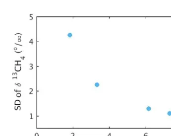
Figure 4.Standard deviation (SD) of the CH4isotopic ratio during the test results shown in Fig. 5.
With the flow rate of 0.400 sccm for the isotopic standard bottles, the total volume of standard gas used was 88 cc. Ob-servations were collected at∼0.5 Hz, and the final 5 min of data for each dilution were averaged to compare against the target value. The standard deviation of the raw data collected during these tests (Fig. 4) decreases exponentially with in-creasing mole fraction.
higher mole fractions, this offset is fairly constant, but for near-ambient mole fractions it is analyzer-specific. We note that the precision of these results could be improved by av-eraging over longer periods. We now describe the calibration technique to remove these offsets.
4.2 Application of calibration equations
The first step in the calibration process for the analyzers is to remove the nearly linear error that is a function of isotopic ra-tio. We applied methods leading from the theoretical frame-work developed by Rella et al. (2015) to calibrate the isotopic ratio data. Applying a linear fit to highest mole fraction val-ues (7.3 ppm) measured in the laboratory for knownδ13CH4 values (−23.9,−38.3,−54.5,−66.5 ‰) for each analyzer, we determined the linear calibration coefficientsp1andp0.
h
δ13CH4
i
intermediate
=p1
h
δ13CH4
i
measured
+p0 (2)
For this step, we used only the highest mole fraction values because δ13CH4 is more precise for higher mole fractions (Fig. 4). We note that these laboratory tests were completed prior to the Allan standard deviation testing and that the av-eraging times were not sufficient to achieve the desired com-patibility at ambient mole fractions. Ambient mole fractions could be used for this step if measured for sufficient dura-tions.
To correct for the CH4mole fraction dependence of the measured δ13CH4, the two time-dependent drift parameters described in Rella et al. (2015), c0 andχ, must be deter-mined. Here c0 varies because of spectral variations in the optical loss of the empty cavity, andχ varies because of er-rors in the temperature or pressure of the gas, or changes in the wavelength calibration. These parameters are defined in Eq. (15) of Rella et al. (2015). A coefficient describing the changes in the crosstalk between the two methane isotopo-logues was ignored, following Rella et al. (2015). For the laboratory calibration, we determinedc0 andχ using mea-surements at−23.9 ‰ for a high mole fraction (7.3 ppm) and a low mole fraction (1.8 ppm). We then applied Eq. (12) of Rella et al. (2015),
h
δ13CH4
i
calibrated
=
h
δ13CH4
i
intermediate
+ c0 c12
+χhδ13CH4
i
intermediate
−B, (3)
to correct for the CH4mole fraction dependence ofδ13CH4. Herec12is the measured [12CH4], and
B=p1Bdefault+p0, (4)
withBdefault being −1053.59 ‰.Bdefault is the intercept of the fit of the isotopic ratio to the ratio of the absorption peak heights for the standard calibration, and B is the up-dated value, specific to the analyzer. We followed Rella et
al. (2015) and ignored the contribution of an additional off-set term that depends on neither mole fraction nor isotopic ratio. Note that the slope of the linear calibration was the only component of the calibration that was not adjusted in the field using field tanks (Sect. 5.4).
5 Methods: field deployment
5.1 In situ field tanks
At each tower site, three field tanks were utilized, as listed in Table 1. One tank at each tower site was calibrated by NOAA for CH4and CO2mole fractions and by the Institute of Arctic and Alpine Research (INSTAAR) forδ13CH4. This tank was tested quasi-daily (every 21 h) and used to adjust the intercept for the CH4and CO2mole fraction calibrations (Richardson et al., 2017). The constituents of this tank were at typical ambient levels (as listed in Table 1); for the purposes of this paper, we call it the “target”, although it was not independent. Two additional tanks were tested at each of the tower sites (Table 1). Scott Marrin, Inc., filled these tanks using ultra-pure air spiked with high methane air from Isometric Instru-ments, Inc., bottles. The resulting mixtures contained 1.9– 2.1 ppm CH4at−23.9 ‰δ13CH4and 9.7–10.5 ppm CH4at
−38.3 ‰δ13CH4). Recall that these are called the “low” and “high” tanks, for simplicity. These tanks contained ambient levels of CO2(368–407 ppm). The choice of the CH4mole fraction of the high tank is based on the optimal determina-tion of the calibradetermina-tion coefficientsc0 andχ, rather than the expected range of ambient CH4mole fractions. The effect of
c0on the calibrated isotopic ratio is largest at low mole frac-tions, whereas the effect ofχis independent of mole fraction. Thus the ratio of the high- and low-tank mole fractions deter-mines how separable the two effects are. We therefore chose the high-tank mole fraction to be as high as possible without introducing other nonlinearities into the system.
The high and low tanks for each tower were calibrated forδ13CH4 in the laboratory prior to deployment. First we applied a linear calibration forδ13CH4using measurements from each of four Isometric Instruments bottles (−23.9,
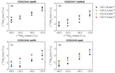
re-Figure 5.Measured isotopic ratio error as a function of known isotopic ratio for each of the four analyzers(a–d),prior to calibration. The colors indicate the12CH4mole fraction, as shown in the legend. The serial numbers (FCDS2046, FCDS2047, FCDS2048, and FCDS2049) of the analyzers are indicated as well. These analyzers were deployed at the south, central, north, and east towers, respectively. Interpolating from the Allan standard deviation results (Fig. 2), the estimated precision is 0.40 ‰ for the 1.80–1.82 ppm CH4 tests, 0.34 ‰ for 3.28– 3.32 ppm CH4tests, 0.24 ‰ for 6.10–6.16 ppm CH4tests, and 0.20 ‰ for 7.26–7.32 ppm CH4tests.
ported by the supplier (Isometric Instruments, Inc.), and in-sufficient testing times for the tanks at ambient mole fractions (5 min). We note that it would have been preferable to utilize calibration tanks closer to the observed air samples in terms of isotopic ratio. In particular, the low tank could have been spiked with the−38.3 ‰ bottle, or a mixture of the−38.3 and−54.5 ‰ bottles.
5.2 In situ field calibration gas sampling system
The flow diagram of the field calibration system is shown in Fig. 6. Polyethylene/aluminum composite tubing (1/4 in. (0.64 cm) OD, Synflex 1300, Eaton Corp.) was used to sam-ple from the top of each tower for the CRDS analyzer, and a separate sample line made from 3/8 in (0.95 cm) OD Syn-flex 1300 tubing was used for the flask sampling packages. The top end of each tube was equipped with a rain shield to prevent liquid water from entering the sampling line. For the CRDS analyzer, air was drawn down the tube at 1 L min−1, with 30 cc min−1flow into the analyzer, and the remainder purged. The residence time in the tube was about 1 min. Sep-arate tubes were used for the CRDS and flask sampling lines because of the differing flow rates required for the flask sam-ples (varying between 0.29 and 3.8 L min−1; Turnbull et al., 2012) and to ensure independence of the CRDS and flask measurements.
For the continuous in situ measurement system, switching between sample and calibration gases was accomplished us-ing a six-port rotary valve (EUTA-2SD6MWE, Valco Instru-ments Co, Inc.). Stainless steel tubing (1/8 in. (0.32 cm) OD, TSS285-120F, VICI Precision Sampling, Inc.) and single-stage regulators (Y11-C444B590, Airgas, Inc.) were used for testing the field tanks. Rella et al. (2015) noted that the ef-fect of water vapor on the isotopic ratio of methane measure-ment is up to 1 ‰ and nonlinear, and recommended drying to less than 0.1 % H2O mole fraction. Thus we used a Nafion dryer (MD-070-96S-2, PermaPure) in the reflux configura-tion, with an additional pump (ME1, Vacuubrand, Inc.) on the outlet of the Nafion dryer (Fig. 6). The sample air was dried to∼0.06 % H2O, and the calibration gases were hu-midified to 0.02 % H2O, in a manner similar to Andrews et al. (2014). The CH4mole fraction was corrected for water va-por following Rella et al. (2015, Supplement), and the CO2 mole fraction following Chen et al. (2010).
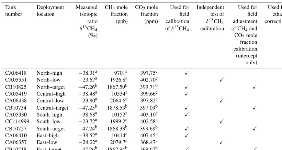
Table 1.Field tanks used at the tower locations. The high and target tanks were used for the field calibration ofδ13CH4. Only the target tank is used for field adjustment of the CH4and CO2mole fraction calibration. The CH4and CO2mole fractions for the high and low tanks are less certain than those of the target tanks.
Tank Deployment Measured CH4mole CO2mole Used for Independent Used for Used for number location isotopic fraction fraction field test of field ethane ratio (ppb) (ppm) calibration δ13CH4 adjustment correction δ13CH4 ofδ13CH4 calibration of CH4and
(‰) CO2mole
fraction calibration (intercept only)
CA06418 North–high −38.31a 9701a 397.75c X X
CA05551 North–low −23.67a 1926.8a 402.70c X
CB10825 North–target −47.26b 1867.59b 399.71b X X X
CA05419 Central–high −38.48a 10534a 399.66c X X
CA06438 Central–low −23.80a 2064.6a 397.82c X
CB10734 Central–target −47.25b 1878.53b 397.09b X X X
CA05330 South–high −38.68a 10152a 403.10c X X
CC114999 South–low −23.72a 1999.2a 402.58c X
CB10727 South–target −47.24b 1868.33b 399.68b X X X
CA06410 East–high −38.52a 10414a 407.45c X X
CA06357 East–low −24.02a 2079.7a 368.47c X
CB10718 East–target −47.26b 1867.94b 399.67b X X X
aDetermined via laboratory measurements.bNOAA/INSTAAR calibration (WMO X2004A scale for CH
4and WMO X2007 for CO2).cField calibration – values not used.
CRDS
Pump (Vacuubrand ME1)
Pump (Vacuubrand ME1)
Na fion
30 sccm
6 port dead-end, common outlet flow path selector
(Valco EUTA -2SD6MWE) Ambient inlet
XHI, δamb
XLo1, δamb
XLo, δheavy
30 sc cm
30 sccm
30 sccm
30 sc cm ~1 LPM
30 sccm Needle valve
Figure 6.Flow diagram of the field calibration system. At standard pressure and temperature, the gas volume of the field tanks was 4021 L.
this time, the CO2 and CH4 mole fractions stabilized. The ideal calibration tank testing time is a balance between min-imizing calibration gas usage (and consequently maxmin-imizing ambient air sampling time) and achieving sufficient preci-sion. Note that the Allan standard deviation results indicate that testing for 4 min for the high tank and for 32 min for the low and target tanks is required to achieve our target
The flow rate of the instruments was 35 cc min−1, and the 150A tank size was used, corresponding to 4.021×10⁶cc at standard pressure and temperature. Thus there was sufficient gas to test each tank for about 1 h per day for about 5 years, as a general guideline.
5.3 Cross-interference from other species
5.3.1 Overview
The effects of cross-interference from other species must be considered for spectroscopic measurements. Rella et al. (2015) give proportional relationships for cross-interference from various species for the G2132-i analyz-ers. Listed in Table 2 are species with potential to affect the isotopic methane calibration and their estimated effects for tower-based applications. We based these estimates on typ-ical maximum values determined by flask (level at which 99 % of flask measurements at the south and east towers were below; for carbon monoxide, propane, butane, ethylene, and ethane), by in situ measurements at the towers in this deploy-ment (for water vapor and carbon dioxide), and by typical values (Warneck and Williams, 2012; for ammonia and hy-drogen sulfide). There are no known ambient estimates for methyl mercaptan (Barnes, 2015), so the odor threshold (De-vos et al., 1990) was used as a maximum value.
For the Picarro G-2132i analyzers, ethane contributed the largest interference, and a correction to the isotopic ratio was applied (Sect. 4.4.2). Because of water vapor effects, the sample was dried, and the calibration gases were humidified. The effects of other species were neglected.
5.3.2 Ethane correction
Ethane (C2H6)is co-emitted with methane during natural gas extraction, and its cross-interference with the isotopic ratio of methane is significant. The magnitude of the effect of ethane on the isotopic methane is proportional to its mole fraction and inversely proportional to the methane mole fraction. The two Scott Marrin field tanks at each site were scrubbed of alkanes (including ethane), but the one NOAA/INSTAAR field tank at each site contained ambient levels of these species. Typical mole fractions of C2H6(1.3 ppb) compared to the Scott Marrin tanks containing no ethane would lead to a 0.04 ‰ bias if uncorrected. Furthermore, flask measure-ments at the south and east towers indicated ethane up to 8 ppb, which corresponds to a 0.23 ‰ error.
The G2132-i analyzers reported an ethane measurement but were not designed for high-compatibility C2H6 measure-ments at levels near background. In this deployment, 99 % of the flask measurements, which were taken in the afternoon, were less than 8.0 ppb C2H6. In comparison, the drives near natural gas sources conducted by Rella et al. (2015) indicated C2H6mole fractions up to 13 ppm (note unit change). The ethane signal is subject to strong cross-interference from
wa-ter vapor, methane, and carbon dioxide. Rella et al. (2015; Eq. S20) report coefficients for these corrections. These co-efficients indicate corrections larger in magnitude than the ethane mole fractions measured in this deployment. We have thus not attempted to analyze the ethane results themselves. The ethane output was, however, used to correct the isotopic methane data. To do so, we first developed a linear calibra-tion using the Scott Marrin high field tank containing zero ethane and the NOAA/INSTAAR target tank which we as-sumed contained a background level of 1.5 ppb ethane (Peis-chl et al., 2016). This calibration is clearly a rough estimate. Note that we determined the linear relationship between the reported ethane of each analyzer and its calibrated value ini-tially, and assumed that this relationship does not change throughout the deployment. Newer models of theδ13CH4 an-alyzer (G2210-i, Picarro, Inc.) measure C2H6at ppb levels, simplifying this correction process.
We then corrected the isotopic methane for the effects of ethane cross-interference. For example, 1.3 ppb of ethane in an air sample of 2 ppm CH4 would, if uncorrected, shift the δ13CH4 measurement higher by [+58.56 ‰ ppm CH4(ppm C2H6)−1×[0.0013 ppm C2H6]/[2 ppm CH4]=
+0.04 ‰. Note that the calibration coefficient for ethane has been updated from that indicated in Rella et al. (2015). The correction to compensate for this error was applied to all data, using the estimated ethane and measured methane val-ues.
5.3.3 Water vapor and carbon dioxide
Water vapor can have a significant effect on the measure-ments of isotopic methane (up to±1 ‰ for up to 2.5 % H2O; Rella et al., 2015). Thus, the sample air was dried and the calibration gases were slightly humidified such that this ef-fect is minimized (estimated to be < 0.02 ‰). For the range of ambient CO2observed in this study (∼375–475 ppm), the difference from the calibration gases was∼100 ppm, and the effect was estimated to be < 0.03 ‰ (Table 2). The isotopic ratio of methane was thus not corrected for CO2effects. 5.3.4 Oxygen, argon, and carbon monoxide
The ambient variability in oxygen, argon, and carbon monox-ide is expected to have a negligible effect on the isotopic ra-tio measurements (Rella et al., 2015), and no correcra-tions for these constituents were applied to the isotopic methane data.
5.3.5 Other species
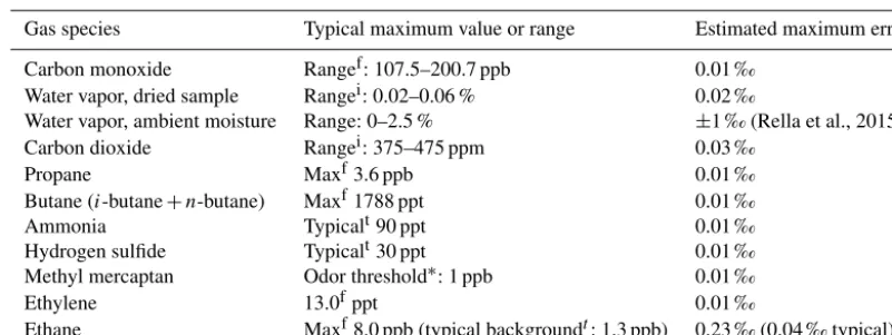
Table 2.Maximum error estimate attributable to cross-interference due to direct absorption onδ13CH4. These estimates were based on typical values for this tower-based application and estimated effects on CRDS measurements (Rella et al., 2015), and assumed 2 ppm ambient CH4 mole fraction. For water vapor and carbon dioxide, the interferences are independent of CH4mole fraction for 1–15 ppm. For the other species listed, the interferences are inversely proportional to CH4mole fraction. Typical maximum values determined by flaskf (level at which 99 % of (afternoon) flask measurements at the south and east towers are below), by in situ measurements at Marcellus towersi, or by typical valuest(Warneck and Williams, 2012).
Gas species Typical maximum value or range Estimated maximum error
Carbon monoxide Rangef: 107.5–200.7 ppb 0.01 ‰ Water vapor, dried sample Rangei: 0.02–0.06 % 0.02 ‰
Water vapor, ambient moisture Range: 0–2.5 % ±1 ‰ (Rella et al., 2015)
Carbon dioxide Rangei: 375–475 ppm 0.03 ‰
Propane Maxf3.6 ppb 0.01 ‰
Butane (i-butane+n-butane) Maxf1788 ppt 0.01 ‰
Ammonia Typicalt90 ppt 0.01 ‰
Hydrogen sulfide Typicalt30 ppt 0.01 ‰
Methyl mercaptan Odor threshold∗: 1 ppb 0.01 ‰
Ethylene 13.0fppt 0.01 ‰
Ethane Maxf8.0 ppb (typical backgroundt: 1.3 ppb) 0.23 ‰ (0.04 ‰ typical)
∗No known ambient estimates (Barnes, 2015)/odor threshold (Devos et al., 1990).
Table 3.Results for the four Marcellus towers using two possible calibration schemes. Tank errors are shown for using the high and low tank in the calibration (scheme A) and using the high and target tank in the calibration (scheme B). The third set of results are for scheme B, but following the change in field tank testing times on 3 December 2016. Results are from October 2016 for the south, east, and north towers but are from May 2016 for the central tower, as the analyzer was at the manufacturer for repairs during October 2016. Note that the daily means of the field tanks are used in the calibrations.
Tower High-tank error (‰) Low-tank error (‰) Target-tank error (‰) mean±standard mean±standard mean±standard deviation for one month deviation for one month deviation for one month (standard error) (standard error) (standard error)
Scheme A South Used in cal Used in cal −0.3±0.4 (0.1) Scheme A East Used in cal Used in cal −0.8±0.5 (0.1) Scheme A Central Used in cal Used in cal −0.5±0.3 (0.1) Scheme A North Used in cal Used in cal −0.4±0.7 (0.1) Scheme B South Used in cal 0.2±0.7 (0.0) Used in cal Scheme B East Used in cal 0.7±0.6 (0.0) Used in cal Scheme B Central Used in cal 0.4±0.5 (0.0) Used in cal Scheme B North Used in cal 0.3±1.3 (0.1) Used in cal Scheme B∗ South Used in cal 0.3±0.3 (0.0) Used in cal Scheme B∗ East Used in cal 0.6±0.5 (0.0) Used in cal Scheme B∗ Central Used in cal 0.4±0.3 (0.0) Used in cal Scheme B∗ North Used in cal −0.4±0.9 (0.0) Used in cal
∗Following change in field tank testing times on 3 December 2016.
of these gases on the isotopic methane is proportional to the mole fraction of the contaminant species and inversely proportional to the methane mole fraction. In Table 2, max-imum mole fractions from the flasks if available, or typi-cal mole fractions from the literature, were used to estimate the effect of these species for our application. The cross-interference from these species was insignificant for our ap-plication, < 0.01 ‰.
5.4 Field calibration
Figure 7. Results following isotopic ratio laboratory calibration only (black) and following calibration (blue) for the south tower for September–December 2016 for the “high” CH4mole fraction tank(a), “low” CH4mole fraction tank(b), and target tank(c). The target tank was used in the isotopic ratio calibration, whereas the low tank was independent. An improved calibration tank sampling strategy was implemented on 3 December 2016 (indicated by ver-tical dashed lines). The Allan deviation for the time period used for each calibration cycle was, for the period prior to the improved tank sampling strategy, 0.2 ‰ for the high tank and 0.5 ‰ for the low and target tanks. Following the implementation of the improved tank sampling strategy, the Allan deviation for each calibration cy-cle was 0.1 ‰ for the high tank and 0.3 ‰ for the low and target tanks.
was calculated using all of the calibration cycles during the month. The errors near the isotopic ratio of the target tank are likely less in magnitude. Instead using the low tank in the calibration and keeping the target tank independent yielded similar magnitudes of errors (Table 3, scheme A) but min-imized bias near the low tank (about −23.9 ‰) rather than near the target tank (about−47.2 ‰). Therefore, despite in-creased testing of the low tank throughout the majority of the deployment, we chose to use the target tank in the calibration to minimize errors near-ambient isotopic ratios.
On 3 December 2016, an improved tank testing strat-egy was implemented, in which the target tank testing time was increased from 6 to 54 min day−1(excluding transition times), achieved by sampling for 20 min every 420 min cy-cle (3.4 times day−1, on average). The calibration times were completed using multiple cycles in order to avoid not sam-pling the atmosphere for long periods and to measure possi-ble changes in analyzer response throughout each day. The low tank was tested using an identical strategy (20 min ev-ery 420 min cycle), with the total amount of testing time per
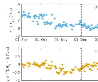
Figure 8.Effect of each of the calibration coefficient terms for the south tower for September–December 2016 for the optimized cal-ibration scheme. The termsc0(a)andχ (b) in Eq. (3) are time-dependent drift terms. Note the differing scales. An improved cal-ibration tank sampling strategy was implemented on 3 December 2016 (indicated by vertical dashed lines).
Figure 9.Low-tank methane isotopic ratio differences from known value, for the individual calibration cycles (blue), and for 1-day (red) and 3-day (black) means of the calibration cycles, for the south tower for September–December 2016. An improved calibra-tion tank sampling strategy was implemented on 3 December 2016 (indicated by the vertical dashed line). The low tank is independent of the isotopic ratio calibration.
day changing from 81 to 54 min. The high tank was tested on average 1.7×per day (every 840 min) for 10 min. Exclud-ing the transition times, the high tank testExclud-ing time was thus reduced from 26 to about 10 min day−1. Following the im-plementation of the improved strategy, the mean error of the independent low tank at the sites was similar, but the stan-dard deviation was reduced from 0.5 to 1.3 to 0.3 to 0.9 ‰ (Table 3).
The relative effects of the calibration terms are illustrated in Fig. 8. The terms c0 (Fig. 8a) andχ (Fig. 8b) in Eq. (3) are time-dependent drift terms. These terms vary because of spectral variations in the optical loss of the empty cavity (c0) and because of errors in the temperature or pressure of the gas, or changes in the wavelength calibration (χ ). Recall that the parametersc0andχwere calculated following Eq. (15) in Rella et al. (2015). The calculation of the parameterc0used measurements from the high and target tank. The calculation of the parameterχ used measurements of the high tank and was not independent fromp0. The largest calibration effect was from thec0term, which increased the calibrated isotopic ratios by−0.5 to 4 ‰ during September to December 2016. Theχterm increased the final calibrated isotopic ratios by a smaller amount,−0.6 to 0.2 ‰. Thus over this period, there were large changes in the calibration effect of these terms, al-though no software or hardware changes were applied. Con-sidering shorter-term changes, the day-to-day changes in the calibration were less than 0.5 ‰ for December 2016. Less frequent calibrations, e.g., twice per week, could be consid-ered, but the reduction in field tank use is not large consider-ing the low flow rates of the instruments and steady changes up to 2 ‰ in the raw data over the timescale of days were observed in Rella et al. (2015).
6 Evaluation of the compatibility of in situ tower measurements
6.1 Independent low tank
The low tank was treated as an ambient sample, indepen-dent of the calibration. To evaluate the noise in the brated ambient samples that results from noise in the cali-bration, we calculated the standard deviation over the period 1 September–2 December of the individual low-tank calibra-tion cycles (6 min each), of the calibracalibra-tion cycles averaged over 1 day (81 min total), and of the calibration cycles aver-aged over 3 days (4.1 h total). These results are a proxy for the noise in the calibrated ambient samples over those testing periods.
The low-tank differences from known values, averaged over differing intervals, are shown in Fig. 9. The standard de-viation of individual low-tank calibration cycles (6 min each) over the period 1 September–2 December is 0.62 ‰. During this period, the calibration used 6 min day−1measurements of the target tank. The standard deviation of the low-tank calibration cycles was similar to expectations based on the Allan standard deviation (Fig. 2). The low tank was tested a total of 81 min (1.35 h) per day. Thus calculating the stan-dard deviation of the low-tank values averaged over each day is a measure of the noise due to the calibration scheme for hourly averages of sample data. The standard deviation of daily averages for the low tank (81 min total) was 0.40 ‰. Based on this result, differences in the hourly average
be-tween towers of less than 0.40 ‰ were likely not significant. For 3-day means (a total of 4.1 h), the standard deviation over the 3-month period was 0.26 ‰. For the period after the calibration tank sampling scheme was improved (primar-ily by sampling the target tank for 54 min day−1instead of 6 min day−1), 3–31 December, the standard deviation of the individual cycles reduced substantially, to 0.25 ‰, and that of the 81 min (4.1 h) mean of the cycles was 0.18 ‰ (0.11 ‰). Therefore, according to this metric, after the improved cali-bration scheme was implemented, differences in the hourly average between towers of greater than 0.18 ‰ were signifi-cant.
6.2 Round-robin testing
Post-deployment round-robin style tests were completed in the laboratory in March 2017 for three of the analyzers, to assess the compatibility achievable via our calibration method. The analyzer deployed at the south tower was not included in these tests, as it was still in the field. Two NOAA/INSTAAR tanks (JB03428: −46.82 ‰ δ13CH4, 1895.3 ppb CH4, and 381.63 ppm CO2; JB03412:−45.29 ‰
δ13CH4, 2385.2 ppb CH4, and 432.71 ppm CO2) were tested and treated as unknowns. The uncertainty for these NOAA tertiary standards was 0.1 ppm CO2, including scale transfer (Hall, 2017; Zhao and Tans, 2006), and 1 ppb CH4(GAW Report No. 185, 2009). The reproducibil-ity based on the calibration results was 0.06 ppm CO2 and 0.4 ppb CH4. The isotopic ratio was tied to the VPDB scale but was not an official calibration (S. E. Michel and B. V. Vaughn, personal communication, 2015). The precision of the determined values assigned to the tanks was 0.04 ‰ (https://instaar.colorado.edu/research/labs-groups/ stable-isotope-laboratory/services-detail/). High, low, and target tanks were tested, with the calibration applied as in the field for ambient samples (as described in Sect. 5.4). The high mole fraction tank was tested for 20 min, and the all ambient mole fraction tanks were tested for 70 min, with 8 min ignored after each gas transition. Four to six tests were completed for each analyzer. We used these tests as a means of evaluating the compatibility of the analyzers, in terms of both mole fractions and the isotopic ratio.
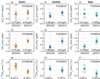
The results for the round-robin style laboratory testing are shown in Fig. 10. The mean of the errors (measured – NOAA known value) for each analyzer–tank pair was−0.08 to 0.04 ppm CO2, within the 0.1 ppm WMO compatibility
Figure 10.Results from round-robin style testing using two NOAA/INSTAAR tanks (JB03428:−46.82 ‰δ13CH4, 1895.3 ppb CH4, and 381.63 ppm CO2; JB03412:−45.29 ‰δ13CH4, 2385.2 ppb CH4, and 432.71 ppm CO2)for CO2(a, b, c), CH4(d, e, f), andδ13CH4(g, h, i)for the analyzer deployed at the north tower (serial number FCDS2048;a, d, g), at the central tower (serial number FCDS2047;b, e, h), and at the east tower (serial number FCDS2049;c, f, i). These tests were completed in the laboratory, post-deployment (March 2017). The analyzer deployed at the south tower (serial number FCDS2046) was not included in these tests. Open circles are individual tests, and filled circles are the means of the individual tests for each analyzer/constituent. The mean error for each analyzer/tank/constituent is indicated in the plots.
tank measuring 2385.2 ppb, and −0.83 to −0.70 ppb CH4 for the NOAA/INSTAAR tank measuring 1895.3 ppb CH4. Therefore, there was a slight error in the slope of the linear calibration, possibly attributable to tank assignment errors. However, the error was well within the WMO recommen-dations for global studies of 2 ppb CH4(GAW Report No. 229, 2016), and the range of NOAA/INSTAAR tanks encom-passed the majority of the CH4mole fraction observed during the study. We also note that the standard error for the means of the CH4 tests was 0.07–0.12 ppb. When averaging over the two round-robin tanks, the mean difference was −0.40 to−0.32 ppm CH4for the analyzers. Forδ13CH4, the mean errors for each analyzer–tank pair were−0.33 to 0.24 ‰ for these tanks, i.e., within the range of ambient isotopic ratio, and the standard errors were 0.05–0.10 ‰. The mean errors were−0.14 to 0.03 ‰ for each analyzer.
6.3 Side-by-side testing
The precision and drift characteristics are not optimized for CO2for the G2132-i analyzers, compared to the G2301 and G2401 analyzers, which measure mole fractions and not iso-topic ratios. Whereas the spectral line for CH4 is the same
between the two types of analyzers (Rella et al., 2015), for CO2, the absorbance of the spectral line used in the G2132-i analyzers is a factor of 11×less, meaning the precision is dramatically reduced. Although not central to the primary results of this project, the performance of the analyzers in terms of CO2is important if the data are to be used as part of the continental-scale CO2network. To test the performance of the G2132-i analyzers for consideration of the data for this use, G2301 and G2132-i (Picarro, Inc.) analyzers were run side by side for 1 month (June 2016) at the south tower. The sampling system for the G2132-i was as described in Sect. 5.2. A separate 1/4 in. (0.64 cm) tube was used for the G2301 analyzer, and an intercept calibration using the target tank was applied daily. The sample air for the G2301 ana-lyzer was not dried, and the internal water vapor correction was used.
Figure 11.Afternoon in situ to flask differences for January–December 2016 for the east (blue) and the south towers (orange) for(a)CO2, (b) CH4, and(c)δ13CH4. For CH4, data points with high temporal variability (standard deviation of raw∼2 s data within the 10 min segments > 20 ppb) are indicated by “+” symbols and have been excluded. The standard deviation of the in-situ-to-flask differences are shown in parentheses on each plot. The standard errors, indicating an estimate of how far the sample mean is likely to be from the true mean, is 0.24 ppb CH4, 0.03 ppm CO2, and 0.06 ‰ at the east tower and 0.14 ppb CH4, 0.04 ppm CO2, and 0.04 ‰ at the south tower.
of the G2132-i is similar for CO2and CH4mole fractions, at least in terms of the long-term mean. In terms of utiliz-ing the mole fraction data in atmospheric inversions, the multi-day mean afternoon differences are most appropriate. The 5-day mean afternoon difference for the month was 0.05±0.08 ppm CO2and−0.7±0.1 ppb CH4. The G2132-i analyzers are thus appropriate for use in the atmospheric inversions and in the global network where 0.1 ppm CO2 and 2.0 ppb CH4have been identified as criteria. For these results, recall that the target tank was tested for a total of 30 min in 5 days. To optimize results on a daily timescale, sampling the target tank for 60 min per day would be preferable for improving CO2 results. We also note that round-robin testing of these instruments requires 60 min sampling per tank.
6.4 Flask to in situ comparison
In addition to the continuous G2132-i analyzers, the east and south towers were also equipped with NOAA flask sampling systems (Turnbull et al., 2012). These flask measurements were used for independent validation and error estimation of the continuous CO2, CH4, andδ13CH4in situ measure-ments. In addition, the flasks were measured for a suite of species including N2O, SF6, CO, H2 (Dlugokencky et al., 2017), halo- and hydro-carbons (Montzka et al., 1993), and stable isotopes of CH4 (Vaughn et al., 2004). The flasks were filled over a 1 h time period in the afternoon (14:00– 15:00 LST), thereby yielding a more representative measure-ment than most flask sampling systems, which collect nearly instantaneous samples (e.g.,∼10 s). Samples were collected only when winds were blowing steadily out of the west or north (∼45–225◦) to ensure that the samples were sensitive to and representative of the broader Marcellus Shale gas pro-duction region that is the focus of this study. For the in situ data, 10 min segments were reported. These were averaged over the hour for comparison with the flask measurements. For CH4, data points with high temporal variability
(stan-dard deviation of the 10 min means within the hour > 20 ppb) were excluded, on the basis that the ambient variability was large, making comparisons difficult.
For January–December 2016, the mean flask-to-in-situ CH4 difference at the east tower was −1.2±2.2 ppb CH4, and at the south tower it was−0.9±1.4 ppb CH4(Fig. 11a). Here the standard deviation reported is that of the hourly flask-to-in-situ differences. Thus, at the south tower, for ex-ample, 67 % of the sampled afternoons indicated differences for CH4within 1.4 ppb of the mean of−0.9 ppb. The stan-dard error was 0.24 ppb at the east tower and 0.14 ppb at the south tower. Thus, there is high confidence that the difference between the in situ and flask measurements at both towers is more compatible than the WMO recommendation. As for the side-by-side testing, the G2132-i analyzers were slightly lower than the “known”, in this case, the flask results. The difference was, however, less than the target compatibility, and the flasks could in theory be biased.
Although CO2 is not the focus of this paper, the dif-ferences were −0.21±0.31 ppm for the east tower and 0.21±0.35 ppm for the south tower (Fig. 11b). The standard error was 0.03 ppm at the east tower and 0.04 ppm at the south tower. The magnitude of CO2differences was some-what larger in the growing season. The mean flask-to-in-situ differences were thus larger than the WMO recommendation of 0.1 ppm, but at the extended compatibility goal of 0.2 ppm CO2(GAW Report No. 229, 2016).
Figure 12.Map of Pennsylvania with permitted unconventional nat-ural gas wells (magenta dots) and network of towers with methane and stable isotope analyzers (Picarro G2132-i). The east and south towers were also equipped with NOAA flask sampling systems. The Binghamton airport is also indicated.
mean error of the independent low tanks (averaging over all calibration cycles during a 1-month period) at the towers (Ta-ble 3) was 0.2–0.7 ‰.
7 Network comparisons
7.1 Study area
Four CRDS isotopic CH4analyzers (G2132-i, Picarro, Inc.) were deployed on commercial towers 46–61 m a.g.l. in north-east Pennsylvania (Fig. 12). The south and north towers were located on the southern and northern edges of the uncon-ventional gas well region, respectively, and were intended to measure background values depending on the wind direc-tion. Measurements began in May 2015, but a complete set of field tanks necessary for calibration ofδ13CH4was not de-ployed until January 2016. The central tower measured only mole fractions for the period June–December 2016. For inter-tower comparisons, we focused on the period January–May 2016, when all sites measured both CH4andδ13CH4. Raw and hourly averaged, calibrated data files are available on-line (Miles et al., 2017).
7.2 Inter-network differences in CH4andδ13CH4
A background value is required to calculate differences in CH4andδ13CH4. For this simple analysis, we chose a single tower to represent the background for the entire period. The predominant wind direction for the Marcellus region is from the west (Fig. 13). For westerly winds, the south tower is a reasonable choice for a background tower. The south tower measured the lowest overall mean afternoon methane mole fraction (1960.2 ppb CH4). The mean afternoon methane mole fractions of the other towers, averaged only when data for the south tower exist, were 8.7, 7.0, and 2.9 ppb higher
Figure 13.Wind rose for surface station at Binghamton, NY, air-port for the period April 2015–April 2016 (using the mean of the afternoon hours for each day). The magnitude of wedges indicates relative frequency for each wind direction, and the wind speeds are indicated by color. These afternoon means were based on hourly reported measurements. For the hourly measurements, calm winds (< 1.6 m s−1)were not categorized by direction and thus were not included in the afternoon mean. For the hourly measurements, calm winds (< 1.6 m s−1)were reported as zero and were included in the afternoon mean.
at the north, central, and east towers, respectively. For fu-ture analysis, a wind-direction-dependent background tower (south or north) could be considered, but the north tower did have the largest mean enhancement in CH4 mole frac-tion as compared to the south tower. As noted by Barkley et al. (2017), the area encompassing southwestern Pennsyl-vania and northeastern West Virginia contains large sources of CH4, with emissions from conventional gas, unconven-tional gas, and coal mines all having significant contributions to the total. These large sources complicated the interpre-tation of the signals, as does changing wind direction. For this overview analysis, we calculated differences above the south background tower to determine overall signal strength to compare with our target compatibility. We first examine the afternoon (defined here are 17:00–20:59 UTC), when the atmospheric is well mixed, allowing simpler interpretation of the measurements and more tractable modeling. We then consider non-afternoon hours, when the atmosphere is less mixed and signals are typically larger.
Figure 14. Probability distribution function of measured isotopic ratio differences from the background south tower (1δ13CH4)for the (a)north,(d)central, and(g)east towers for afternoon hours (17:00–20:59 UTC, 12:00–15:59 LST). The averaging interval of the individual data points for all plots is 10 min, and the time period is January–May 2016. The bin size for (a), (d), and (g)is 0.2 ‰. The median and standard deviation of the differences are indicated on the plots. Probability distribution function of measured methane mole fraction enhancements (1CH4)for the(b)north,(e)central, and(h)east towers. Note that the scale for(b),(e), and(h)has been truncated to focus on majority of the data points. The bin size is 10 ppb CH4. Keeling plots for the(c)north,(f)central, and(i)east towers. The black box in each plot indicates the approximate scale of the corresponding isotopic ratio difference and methane mole fraction enhancement plots. The median and standard deviation of the isotopic ratios at each tower are indicated on the plots. Note that the Allan deviation for 10 min means at ambient mole fractions was 0.4 ‰, and this decreases with increasing mole fraction.
mole fraction (less than 1 ppb) were less in magnitude than the compatibility of the analyzers. This result is generally consistent with the results of Barkley et al. (2017), who found the emission rate of methane due to natural gas extraction ac-tivities to be very low, 0.36 % of total production. The stan-dard deviation of 10 min segments of isotopic ratio differ-ences was 0.8 ‰ at each of the towers. We note that the Al-lan standard deviation for 10 min averaging times for ambi-ent levels of methane was 0.4 ‰δ13CH4. The standard de-viation of the daily afternoon averages (rather than 10 min averages) was 0.6–0.7 ‰. Thus the observed width of the distribution appears to be persistent throughout the afternoon and not merely measurement noise. For isotopic ratio, 43– 54 %, depending on the tower, of the 10 min segments were greater than 0.6 ‰ in magnitude (3×the target compatibility; Fig. 14a, d, and g) and are thus detectable by the analyzers. The standard deviations of the methane mole fraction dif-ferences were 60.7, 30.0, and 33.8 ppb for the north, central, and east towers, respectively (Fig. 14b, e, and h). Differences greater than 6 ppb CH4in magnitude (3×the target
compat-ibility) were indicated by 57–66 % of the data points for the north, central, and east towers (Fig. 14b, r, and h) and are thus detectable. The majority of afternoon data points indi-cated relatively few local sources of contamination.
There are, however, a few outliers during the time period with large values above the background tower during the afternoon hours (up to 1500 ppb enhancement at the north tower). The isotopic as a function of inverse methane mole fraction at each non-background tower is shown in Fig. 13c, f, and i. While the range of measured isotopic ratios is large, the majority of the 10 min means lie close to the ambient val-ues: the standard deviation of the 10 min means of the mea-sured isotopic ratios during the afternoon was 0.6–0.8 ‰.
out-Figure 15. Probability distribution function of measured isotopic ratio differences from the background south tower (1δ13CH4)for the (a)north,(d)central, and(g)east towers for all times of data excluding the afternoon hours shown in Fig. 14. The averaging interval of the individual data points for all plots is 10 min, and the time period is January–May 2016. The bin size for(a),(d), and(g)is 0.2 ‰. The median and standard deviation of the differences are indicated on the plots. Probability distribution function of methane mole fraction enhancements (1CH4)for the(b)north,(e)central, and(h)east towers. Note that the scale for(b),(e), and(h)has been truncated to focus on majority of the data points. The bin size is 10 ppb CH4. Keeling plots for the(c)north,(f)central, and(i)east towers. The black box in each plot indicates the approximate scale of the corresponding isotopic ratio difference and methane mole fraction enhancement plots. The median and standard deviation of the isotopic ratios at each tower are indicated on the plots. Note that the Allan deviation for 10 min means at ambient mole fractions was 0.4 ‰, and this decreases with increasing mole fraction.
Figure 16.Time series of CH4encompassing one of the eight peaks in CH4at the central tower (DOY 55) for which the Keeling plot ap-proach was applied. The averaging interval of the individual points was 10 min, and periods during which field tanks were sampled were excluded from the plot. The linear fit was calculated using the points clearly within the plume (black dots).
liers, particularly at the central tower (Fig. 15c, f, and e). Ap-plying a best-fit line to all of the data shown in Fig. 14f gave a poor correlation coefficient (r2=0.22) because there were many data points with no local sources.
7.3 Keeling plots
Keeling plots (Keeling, 1961; Röckmann et al., 2016) are used to infer the isotopic ratio of the methane source as the intercept of the best-fit line of the isotopic ratio as a function of the inverse methane mole fraction. We used this approach to estimate the source isotopic ratio of the eight largest peaks observed during non-afternoon hours at the central tower. The time series of CH4encompassing the peak observed on day of year (DOY) 55 is shown in Fig. 16, as an example. The time during which the tower was in the plume was clear (lasting about 1.5 h), and only those points were included in the calculation of the linear fit.
Figure 17.Keeling plots for the central tower for the eight largest peaks in the non-afternoon methane time series. Black lines indicate the best-fit lines. Correlation coefficients (r2), day of year (DOY), andyintercepts are indicated in the plots.
sources contributing to the peaks have a mean isotopic ra-tio of−31.2±1.9 ‰. The correlation coefficients were high (r2=0.92–1.0) except for one peak, which was excluded from the statistics. When propagating a potential error (at-tributable of analyzer uncertainty) of 0.2 ‰ at the heavy end of the Keeling plots and −0.2 ‰ at the light end, and vice versa, the potential range of the mean is from−32.0 to
−30.4 ‰.
Compared to mobile measurements near the ground, for example, the footprints of towers are large, which is ideal for determining regional emissions. But the emissions sources with specific isotopic signatures are diluted by mixing, mak-ing the enhancements above background small, particularly for this region/time period with small leakage rates. For these eight non-afternoon peaks at the central tower, the enhance-ments over background were 334.1–2007.8 ppb CH4, and the differences of isotopic ratio were−2.5 to−8.7 ‰.
8 Discussion
In this paper, we present the methods used to calibrate a network of four CRDS methane isotopic ratio analyzers (Pi-carro G-2132i). Evaluation of the calibration results using an independent tank, round-robin style testing, and flask com-parisons showed that the analyzers are compatible within 0.2 ‰. The calibration required consideration of (1) the iso-topic ratio linear calibration, (2) the mole fraction
Table 4. Possible field tanks and sampling strategies, including those employed in the present study. The “Improved strategy” column suggests a possible strategy in which three field tanks and one independent tank are employed, and thus laboratory calibration is not required. Estimated tank testing times (excluding transition times) are listed for various compatibility requirements.
Present study prior to 3 December 2016
Present study 3 December 2016 and thereafter
Improved strategy
Laboratory calibration needed?
Yes, for linear calibration Yes, for linear calibration No
High CH4mole fraction tank(s)
HIGH (10 ppm, −38.3 ‰, 26 min day−1)
HIGH (10 ppm, −38.3 ‰, 10 min day−1)
HIGH (10 ppm, −38.3 to −44 ‰, 8 min day−1 for 0.1 ‰ Allan deviations, 1 for 0.2 ‰, 1 for 0.4 ‰)
− − HIGH (10 ppm,
−54.5 to−52 ‰, 8 min day−1for 0.1 ‰ Allan devia-tions, 1 for 0.2 ‰, 1 for 0.4 ‰)
Low CH4mole fraction tanks
LOW (2 ppm,
−23.9 ‰, 81 min day−1)
independent
LOW (2 ppm, −23.9 ‰ 54 min day−1) indepen-dent
LOW (2.1 ppm,−46.5 ‰ (ambient), 120 min day−1for 0.1 ‰ Allan deviations, 60 for 0.2 ‰, 8 for 0.4 ‰)
TARGET (2 ppm, −47.2 ‰, 6 min day−1)
TARGET (2 ppm, −47.2 ‰, 54 min day−1)
TARGET (1.9 ppm,−47.5 ‰ (ambient), 120 min day−1 for 0.1 ‰ Allan deviations, 60 for 0.2 ‰, 8 for 0.4 ‰)
independent
Notes Reduced noise in
calibra-tion due to increased tar-get tank testing time
Does not necessarily require laboratory calibration of analyzers. Range of ideal isotopic ratios for the high tanks is given. Utilizing the isotopic ratios of com-mercially available bottles for spiking (i.e.,−38.3 and −54.5 ‰) may avoid the need for laboratory calibration of these tanks. Using the range of the near-ambient iso-topic ratio of low/target tanks (but not exactly the same isotopic ratio, and preferably not exactly the same mole fraction) is more accurate reflection of compatibility, and range of the isotopic ratio of the high tanks better encompasses expected values. For applications with re-duced compatibility requirements (e.g., 0.4 ‰), utiliz-ing low/target tanks at commercially available−38.3 and−54.5 ‰ may be sufficient. It is advantageous to distribute field tank testing throughout the day, to avoid not sampling ambient air for long periods and to mea-sure potential changes in analyzer response.
Our recommendation for future similar studies is to choose both target and low tanks closer to the expected range of isotopic ratios, in addition to being near-ambient CH4mole fractions. For example, suggested values for the low and tar-get tanks are 2.1 ppm CH4 at−6.5 ‰ and 1.9 ppm CH4 at
−47.5 ‰ (Table 4 and Fig. 18b). The testing time required is dependent upon the compatibility goals. After implementing our improved tank testing time strategy, we tested each target and low tank for about an hour per day, to achieve Allan de-viations of 0.2 ‰. Source attribution using mobile measure-ments, rather than tower measuremeasure-ments, for example, is less demanding in terms of compatibility needed, due to the rela-tively large ambient signals typically encountered. The esti-mated testing time required to achieve Allan deviations less than 0.4 ‰, for example, is 8 min. In general, it is desirable to distribute the tank testing time throughout the time period, in our case, 1 day. In this case, persistent changes in analyzer response over the day, if any, would be averaged over rather than an extreme value used in the calibration. This proce-dure also avoids not sampling the ambient air for extended periods. We did not find any evidence of variability in the
calibrations on scales less than 1 day, compared to the preci-sion possible given our tank testing times, but this possibility could be further explored by testing the field tanks for longer periods of time.
im-Figure 18.Graphical representation of the field tanks used in the present study(a), and for an improved strategy (as in Table 4;b). Orange “H” symbols indicate high mole fraction tanks, blue “L” symbols indicate low mole fraction tanks, and red “T” symbols in-dicate target tanks. Lines in(b) indicate range of isotopic values desirable for the high tanks.
portant – improving linear calibration frequency or avoiding over-constraining the calibration.
In this paper, we calibrated the total CH4and the isotopic ratio of methane. An alternative calibration approach is to separately calibrate the individual isotopologues (in this case, 13CH
4and12CH4dry mole fractions), as has been applied to Fourier transform infrared and isotope ratio infrared spec-trometers measuringδ13C andδ18O of CO2 in air (Griffith et al., 2012; Wen et al., 2013; Flores et al., 2017). This ap-proach has the advantage of simple calibration equations but has the disadvantage that the quantities of interest (e.g., to-tal mole fraction and isotopic ratio) are calculated rather than directly calibration. Like the approach applied in this paper, it also requires at least two standard tanks and could utilize an independent tank for testing. Rella et al. (2015) list fur-ther practical reasons to calibrateδ13CH4,including the lack
of primary standards for 13CH4. However, a comparison of performance using each of these techniques on the same data set would be beneficial.
The signals observed in the study region were generally small, but the isotopic ratio differences were larger than would be expected based on the methane mole fraction en-hancements from local sources. For afternoon hours at the central tower, for example, 43 % of the differences inδ13CH4 were detectable above background with magnitudes > 0.6 ‰, 3 times the analyzer compatibility. For a thermogenic source with isotopic ratio of−35 ‰ and a background isotopic ra-tio of −47 ‰, and assuming a measured CH4 mole frac-tion of 2000 ppb, a measured isotopic ratio difference of
−0.6 ‰ corresponds to a 100 ppb peak in CH4above back-ground, following Eq. (1). Enhancements in CH4of 100 ppb were rarely encountered, however (Fig. 14b, e, and h). Using
Eq. (1) to predict differences of isotopic ratio based on the observed methane mole fraction enhancements corresponded to only 3 % of the isotopic ratio differences expected to be > 0.6 ‰ in magnitude. Thus during the afternoon hours, most of the deviations from background were not likely directly from local sources. These larger-than-expected differences in isotopic ratio are not primarily attributable to analyzer noise. The Allan deviation (Fig. 2) is 0.4 ‰ for 10 min means at am-bient mole fractions of 2 ppm CH4. We also note that we fo-cused on the period January–May 2016 in this work. Larger differences were observed in the latter half of 2016.
During the morning hours, however, several peaks result-ing from local sources were observed. The mean source iso-topic signal indicated by Keeling plot analysis of the eight largest peaks at the central tower was−31.2±1.9 ‰, fairly heavy even for oil/natural gas sources. In general, the iso-topic signature for natural gas sources varies from region to region, and even within one region. The mean isotopic ra-tio of methane in gas wells in the northeastern Pennsylvania section of the Marcellus region has been shown to vary by depth, from−43.42 ‰ with a standard deviation of 6.84 ‰ for depths of 0 to 305 m, to−32.46 ‰ with a standard devia-tion of 3.84 ‰ for depths greater than 1524 m (Baldassare et al., 2014). Similarly, Molofsky et al. (2011) found that the isotopic signatures of gases from the deeper layers of the Marcellus Shale in Susquehanna County, Pennsylvania, to be heavier than the shallower Middle and Upper Devonian de-posits, with values for the deep layers ranging from−30 to
−21 ‰. Thus, the source signature determined here is con-sistent with a natural gas source originating from deep wells in the Marcellus region. The peaks occurred during the morn-ing hours, when the boundary layer is typically stable, mak-ing modelmak-ing more difficult, and the winds prior to the peaks were not from a consistent direction. Determination of the location of the specific emitter(s) contributing to these peaks is thus beyond the scope of this paper. Based on the lack of consistent wind direction, it seems likely that more than one location (with potentially different source signatures) con-tributed to these peaks. We note that the Keeling plot ap-proach to determine source isotopic signatures far from the point of emission will be difficult to apply in regions without sources that are significantly depleted or enriched in13CH4 compared to ambient.