www.nonlin-processes-geophys.net/18/133/2011/ doi:10.5194/npg-18-133-2011
© Author(s) 2011. CC Attribution 3.0 License.
Nonlinear Processes
in Geophysics
A Barnes-Hut scheme for simulating fault slip
N. M. Beeler1and T. E. Tullis2
1US Geological Survey, Cascades Observatory, Vancouver, Washington, 98683, USA 2Brown University, Providence, Rhode Island, 02712, USA
Received: 26 March 2008 – Revised: 7 January 2010 – Accepted: 1 June 2010 – Published: 4 March 2011
Abstract. To account for natural spatial and temporal com-plexity, large-scale, long-duration calculations are required for simulations of seismicity in fault zones that host large earthquakes. Without advances in computational methods, the rate of progress in “earthquake simulator” models and as-sociated earthquake forecasts is limited by the rates at which computer speed and storage increase. To explore improve-ments in computational efficiency we develop the first im-plementation of the Barnes-Hut algorithm (Barnes and Hut, 1986) to calculate elastic interactions in a fault model. The Barnes-Hut method is an efficient, numerical scheme that treats local forces exactly and distant forces approximately. The approach is illustrated in example simulations of non-linear fault strength in plane strain. Rudimentary error analy-sis indicates that efficient calculations, where execution time scales with number of grid points (N) as NlogN, can be conducted routinely with errors on the order of 0.1%. We ex-pect the Barnes-Hut method to be well suited for conducting initial exploration of parameter space for fault simulations with non-linear constitutive equations, and for efficient cal-culations of stress interaction in complex fault systems.
1 Introduction
A developing field in earthquake hazard research is the con-struction of “earthquake simulators”, deterministic models that are intended to capture the statistical properties of seis-micity in specific natural fault zones. Earthquake simula-tors use as input a particular natural network of faults from the mapped surface and subsurface expression, along with associated recurrence time or long term slip rates as con-strained by paleoseismic and geodetic data (Rundle, 1988a, b; Ward, 1992, 2000; Robinson and Benites, 1995, 1996). These models produce synthetic seismic catalogs but they
Correspondence to: N. M. Beeler ([email protected])
differ from the broader class of non-continuum models that includes cellular automaton (Burridge and Knopoff, 1967; Carlson and Langer, 1989a, b) and other cellular elastic models (Ben-Zion and Rice, 1993, 1995) in that the simula-tor models consider specific faults. The objective of synthetic seismicity models is to reproduce the overall statistical prop-erties of earthquakes, e.g., frequency magnitude relations, in-terevent times or aftershock-foreshock statistics. Thus, the class of models that we refer to as “earthquake simulators” in this paper, such as Rundle (1988a, b), Ward (1992, 2000), Robinson and Benites (1995, 1996), are deterministic models of the occurrence and statistical properties of particular syn-thetic earthquakes within a specific natural fault network. The objective of the simulators is to reproduce the overall statistical properties of specific natural large earthquakes in the fault system of interest.
inclusion in simulator models is huge, suggesting that ad-vances in computational approach are also needed, as fol-lows.
In the temporal domain, natural earthquake clustering (foreshocks, aftershocks) presumably reflects on-fault phys-ical processes that influence event occurrence times. Labo-ratory observations of frictional fault slip and rock fracture can explain some properties of temporal clustering. The key aspect is a small instantaneous dependence of fault strength on sliding rate that is observed during slip on pre-existing faults (Dieterich, 1979) and intact rock failure (e.g., Scholz, 1968a). The consequences of this rate dependence are pro-found; failure occurs following a prolonged period of grad-ual slip acceleration and failure time is somewhat insensitive to stress changes; both effects are due entirely to damping of the slip rate by the instantaneous rate dependence. In particular, time of failure depends on the size of the stress change and the fault’s initial temporal proximity to failure (e.g., Scholz, 1972; Dieterich, 1994), resulting in what is known as “static fatigue” in the rock failure literature, (e.g., Scholz, 1972; Kranz, 1980). When this behavior is attributed to fault populations in model calculations, earthquake occur-rence rates are time-dependent, such that aftershocks (Mogi, 1962; Scholz, 1968b; Knopoff, 1972; Das and Scholz, 1981; Yamashita and Knopoff, 1987; Hirata, 1987; Reushle, 1990; Marcellini, 1995, 1997; Dieterich, 1994, among others) and foreshocks (Das and Scholz, 1981; Dieterich, 1994) are pre-dicted. This class of models does not explicitly consider spe-cific faults or fault geometry. The seismicity rate formula-tion of Dieterich (1994) is the most flexible of this type of synthetic seismicity model.
To incorporate laboratory-observed time-dependent fric-tion rigorously in earthquake simulator models requires nu-merical solution of differential equations. As typical large earthquake periodicities exceed 100 years and require multi-cycle simulations to study recurrence probability, the extent that friction constitutive equations can be applied in earth-quake simulator models is limited by computer speed. Con-sequently, published results from these kind of models to date (Rundle, 1988a, b; Ward, 1992, 2000; Robinson and Benites, 1995, 1996) use rudimentary relations for failure and fault strength (e.g., static-kinetic friction) that lack the inherent time-dependence.
One promising development that allows for time-dependent earthquake occurrence in these earthquake sim-ulations is a fast computational scheme proposed by Di-eterich (1995). The algorithm replaces nonlinear friction constitutive equations with analytical approximations; for the delayed failure described above the scheme uses a simpli-fication that underlies the Dieterich (1994) seismicity rate formula and the precursory slip that accompanies interseis-mic strength recovery (Dieterich, 1972) is ignored. Further-more, seismic fault slip is represented as quasi-static with a limit on slip speed from theory of Brune (1970). This Dieterich (1995) algorithm eliminates the numerical
solu-tion of differential equasolu-tions and thereby reduces computa-tion time by orders of magnitude (Dieterich and Richards-Dinger, 2010). Similar approximations could be developed for other source processes that may operate during dynamic slip, such as pore pressurization, and particularly those that operate during the interseismic period.
In addition to natural temporal effects and the inher-ent computational problems they presinher-ent, the overwhelm-ing complexity of natural seismicity is in the spatial domain (Ben Zion, 2008). Mature natural faults are non-planar and segmented, having finite width and heterogeneous material properties. They are embedded in a heterogeneous and dam-aged elastic crust. Natural fault systems or networks are geo-metrically intricate collections of fault zones, in which there are earthquakes with over 10 orders of variation in moment magnitude. Because of the breadth of scale and geometrical complexity, to date the earthquake simulators are coarse and simplified.
All of the simulators in current use (e.g., Rundle, 1988a, b; Ward, 1992, 2000; Robinson and Benites, 1995, 1996) use analytical static solutions to slip on a dislocation seg-ment (e.g., Chinnery, 1963; Okada, 1985, 1992) to calculate stress interactions between segments. Calculating the static interactions places limitations on computation size or seg-ment density because in 1-D stress at any segseg-ment centerτi
changes due to the sum of slips δj of all source segments j= 1,N as
1τi=Kijδj j=1... N (1)
where the Kij’s are linear elastic stiffness coefficients and
N is the number of fault cells. Calculating stress at each segment requiresN computations for a total ofN2over the entire grid. Thus, there are practical limits on spatial di-mension or segment density in simulations of fault systems due to the computation time and memory requirements in-creasing strongly with the number of fault segments used. In summary, without ignoring some aspects of natural spa-tial or temporal complexity, without using approximate solu-tions or other time saving approaches, the rate of progress in earthquake simulation and associated earthquake forecasting is limited by the rates in which computer speed and storage increase.
(a) (b)
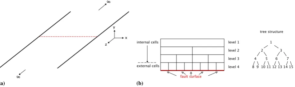
Fig. 1. Fault geometry, cell and tree structure of the plane strain Barnes-Hut implementation. (a) Schematic representation of a fault in a whole space in plane strain. This is the geometry that is used in all the calculations in this paper. The fault is in the plane containing the z and x axes; the y direction is the fault normal. It has a finite length in the x direction and extends infinitely in the positive and negative z directions. The red dashed line, shown for reference, is the intersection of the fault with the plane containing the y and x axes at z = 0. (b) Cell and tree representation of the fault. Left panel shows the fault trace from (a) in red, that is, the intersection of the fault with the plane containing the y and x axes, corresponding to the red dashed line in (a). The fault is divided into 23equi-dimensioned external cells. Above the fault in the left panel are the 23−1 internal cells, labeled by level. Right panel shows the internal and external cells schematically as a tree structure, a choice of corresponding cell numbers, and lines connecting parent to daughter cells.
computer storage and computation time constraints. With-out going into great detail, the strategy of a FMM for dis-location modeling of fault slip would be to combine fault segments and compute interactions with other combined seg-ments which are sufficiently far away from each other using a series expansion of the elastic stiffness coefficients. Interac-tions with segments that are nearby are calculated essentially without approximation. The FMM reduces the number of necessary pair-wise interactions fromN2to orderN (Green-gard and Rohklin, 1987). A method for calculating fault slip based on Warren and Salmon (1993, 1994) has been devel-oped by Tullis and co-workers (Tullis et al., 1999). Though this method is referred to in the literature as a FMM, the num-ber of interactions scales asNlogN, rather than as N and more accurately this is a “tree” algorithm (see below) and not strictly a FMM.
Like the FMM, the Barnes-Hut method is an approximate numerical algorithm that reduces the number of mathemat-ical operations necessary to solve a field problem (gravity, electrical, stress, etc.). Also like the FMM the BHM was used initially to calculate gravitational attraction amongst a large number of bodies (the N-body problem), but it can be used in other problems where the influence of a force de-creases with distance. We develop the first explicit imple-mentation of this method to simulate fault slip. As with the FMM, stress contributions from slip on nearby (local) fault segments are treated using the analytical solution for a dis-location and the stress contribution from the slip of distant segments uses approximate relations. Successful approxima-tion requires that the local region about each segment is se-lected to be large enough to include the fault segments with the predominant stress interactions. The implementation of the Barnes-Hut algorithm is very different from the FMM. It
uses no series expansion of the coefficients of the stiffness matrix K in (1) and it uses a tree computational structure. It is somewhat less efficient than the FMM, reducing the num-ber of pair-wise interactions to orderNlogN, rather thanN. It is, however, considerably simpler to implement relative to the FMM and the implementation is simple in the absolute sense as we hope to convey in this report.
2 The Barnes-Hut method
The Barnes-Hut approximation relies on forces decreasing with distanced between points of application and interest, for example for gravity as 1/d2 (e.g., Turcotte and Schu-bert, 1982). At low cost to accuracy, distant forces have small influence and can be treated less rigorously than the nearby sources with larger influence. Using a gravity ex-ample, rather than calculating the effect of the attraction of each object in a distant galaxy on the Earth, the force of the summed mass of the entire galaxy can be treated as a point source applied its center of mass. The effect of the galaxy on the many other objects distant to it can be calculated in the same way.
Dislocation based faulting programs require the stiffness matrix Kij in Eq. (1), consisting of one coefficient for each
pairwise elastic interaction. These are static stiffness coef-ficients and are applied in earthquake simulators in a quasi-static time stepping routine that ignores elastodynamic wave propagation. The implications of using this quasi-static ap-proximation in earthquake simulators are not well under-stood and this is a topic of active research (Tullis et al., 2009). In this study we also ignore elastodyanmic effects. The Kij
are distance dependent; for plane strain Kij ∝ 1/d2 (see
Eq. 6 below), and for 3-D∝1/d3. The Kij coefficients are
also proportional to the source segment width. The construc-tion of the K matrix, consisting ofN2calculations, is over-head prior to the actual stepping of displacement and stress (1) through time. This overhead is discussed in more detail in Sect. 3.1 below. At each time step in a standard program there are an additionalN2operations, those associated with calculating Eq. (1). The BHM replaces Kij with a smaller
matrix. The result is that at each time step rather than there beingN2operations there are fewer. This is where the time-savings in the method resides. There is overhead associated with setting up the smaller K matrix, but this is time well spent. Accordingly, the Barnes-Hut method consists entirely of constructing a K matrix that is much smaller but that is sufficient to produce an adequate estimate of the stresses due to fault slip. To illustrate the approach we use plane strain where the fault segment influence coefficients decay with distance from the source as in the classic Barnes-Hut grav-ity problem (Barnes and Hut, 1986) and the same decision-making criterion can be used unambiguously.
The computational algorithm uses a tree structure (Fig. 1b). Tree levels are denoted fromk=1 to nn+1, where nn is an integer. The top level of the tree (k=1) is a single cell or segment with length equal to the entire fault. The sec-ond level (k=2) consists of 2 cells of equal width; these are daughter cells of the top-level single parent cell. The third level is constructed by dividing each parent on level 2 into two daughters so that tree levelk=3 has 2(k−1)=4 cells. Sub-sequent levels follow the same procedure. This is a binary tree. The bottom level consists of the actual fault grid ofN
segments. For simplicity the actual fault grid size is uniform
in this example and throughout. Also, to simplify the tree structure, we only consider actual fault grids of integer pow-ers of two,N=2nn, and nn can be used to specify the height of the tree (nn+1) as well as the number of actual fault cells. The actual fault segments are referred to throughout as exter-nal segments or cells. The segments at upper levels of the tree (k <nn + 1) are internal segments.
The smaller BH stiffness matrix K that is analogous to Kij
in (1) is constructed by sequentially traversing the tree struc-ture from the top down for each external segment and com-paring the ratio Dx/Lfor each internal segment to see if it is larger than a chosen value,φ. Here Dx is length of the inter-nal segment, andLis the distance between the center of the internal and the external segments. If Dx/L < φthe internal cell is deemed far enough from the external cell to be treated approximately (distant). An influence coefficient commen-surate with the internal cell’s dimension and distance is used, and all its external and internal daughter cells are excluded from the computation (Fig. 2). If Dx/L > φthe internal cell is too close to the external cell, it is excluded from the com-putation, and 2 or more of its daughter cells will be used in-stead. Using this algorithm, K is generated containing a row for each external segment that consists of the influence co-efficients corresponding to other external cells that are local, and approximate influence coefficients for distant cells. The valueφ= 0 corresponds to the fullN×N Kij matrix in (1),
and larger values to smaller K and increasingly more approx-imate calculations. Stress at each external cell is the product of the appropriate row of the K matrix and the corresponding external segment local values of slip and representative slips associated with the distant internal segments. In this imple-mentation, the internal representative slips are the average of their external daughter segment slips. As a practical matter,
φis greater than or equal 0. Furthermore it also should not be much larger than 1. The long-range elastic interactions that produce coherent nucleation and growth of a simulated earthquake in the calculations in this paper disappear asφ
exceeds 1 (forφ= 1,L= Dx, so even adjacent cells would be excluded from the calculation).
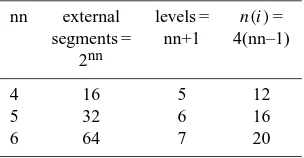
Table 1. The summary of the scaling which isNlogN.
nn external levels = n(i)= segments = nn+1 4(nn–1)
2nn
4 16 5 12
5 32 6 16
6 64 7 20
2.1 Expected speedup and scaling relations
How the number of non-zero entries in K increases with in-creasing grid size or density determines how the duration of calculations scale withN. Scaling can be understood qualita-tively by considering a single cell (red) within the grid struc-ture as the grid extent is increased (Fig. 2); in this example
φ=0.5. As the grid is increased by a factor of two, the cells used (grey) to calculate stress change rather than double, in-crease by only four cells, specifically as 4(nn–1). The grid hasN=2nncells so by assuming that our single example cell is representative, the size of K is approximately 4N(nn-1) = 4N (−1+log2N )=13.3Nlog10N−4N. So for large calcu-lations the scaling isNlogN as in the original Barnes-Hut method (Barnes and Hut, 1986). The fractional increase in execution time of the Barnes-Hut method, the speedup, should scale then asN/logN. The trend in scaling will ex-tend to the practical time and memory limits of available computers. And since speedup is an increasing function ofN, time-savings for large scale simulations should be immense. 2.2 Implementation specific properties
of the Barnes-Hut scheme
Before moving on to the actual calculations a couple of dif-ferences between the problem of fault slip and the classic implementation of the BHM are worth noting. A principal difference is that for the BH gravitation problem the anal-ogous influence matrix K is dynamic. That is, space is di-vided up into a static grid populated by moving bodies; so, an influence coefficient changes with time depending on the particular mass contained within the source grid element. As a consequence, the K matrix has to be recalculated at every time step. In our fault implementation the fault is fixed in space and the off-fault elastic properties are constant so the K matrix is static. K can be set up once and stored, lead-ing to a more efficient method. A downside to this is that in the classic implementation the errors are nearly random and accumulate essentially as a random walk (Barnes and Hut, 1986) whereas for faulting the errors correlate in sign from one time step to the next leading to accumulation and the approximate solution may drift from the actual more rapidly in time.
2.3 Definitions of error and error magnitude that are used in this study
To judge the performance of the BH algorithm we track the errorEassociated with the method by comparing a particular solution at a grid pointxat timetusing the BHM,p(x,t ), to the full solutionf (x,t ), typically, the solution without the BH approximation. Throughout we define error at a grid point as the difference between the solution of the BHM and that of the full solution,
E=f (x,t )−p(x,t ).
f (x,t ) is assumed to be the correct solution. That is, our desire is to characterize how good the BH method is at re-producing the answer that would be otherwise obtained with the full dislocation model. The magnitude of the errorMis characterized using the absolute value of the fractional error,
M=
f (x,t )−p(x,t ) f (x,t )
,
or the percent error, 100∗M. Furthermore, we will refer to
the magnitude of the error as “an error of order. . . ”. For ex-ample an errorM=0.004 would be an error of order 0.001 or an error on the order 0.1%.
3 Geometry and boundary conditions
We apply the method to a fault in plane strain within a whole space (e.g., Weertman, 1979; Dieterich, 1992) (Fig. 1a). The fault is divided into N edge dislocation segments and the stress on segmenti is the sum of an initial stressτi0, stress resulting from self slip and slip of all the other segments1τi,
and a remote uniform (tectonic) stressing
τi=τi0+1τi+ ˙τ t, (2)
wheret is time andτ˙ is the stressing rate. In the complete solution1τi is given by (1). More generally for the BHM
1τi=Kijδj j=1...ni ni≤N (3)
level 1 level 2 level 3 level 4 level 5
level 1 level 2 level 3 level 4 level 5 level 6
level 1 level 2 level 3 level 4 level 5 level 6 level 7
Fig. 2. Schematic construction following the system of Fig. 1b, illustrating scaling as the grid extent increases from 16 to 64 cells. Outlined in red is a particular cell of interest. Gray shaded cells are those whose displacements are used to estimate the red cell’s stress in a BH calculation withφ= 0.5. As the grid extent doubles, the number of gray cells increases by just 4 cells. The Table 1 summarizes the scaling which isNlogN(see text).
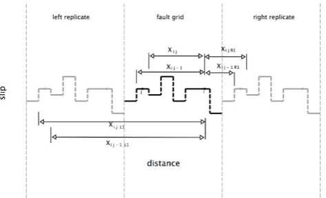
Fig. 3. Example grid, like Dieterich (1992) and Weertman (1979) but with periodic boundary conditions. This grid is used in all cal-culations in the present study. The periodic boundary conditions are used to approximate solutions obtained with an accurate Fourier method (Rubin and Ampuero, 2005).
itself. Influence coefficients consist of two terms for the ac-tual source segment and 4 additional terms for each pair of replicate segments, one added to each side of the fault,
Kij = G
2π (1−υ)
" 1
Xij
− 1
Xij−1
+
( m X
k=1 1
Xij Lk
− 1
Xij−1Lk
+ 1
Xij Rk
− 1
Xij−1Rk
, (4)
wheremis the number of replicate pairs and the distances for a single replicate pair,Xij L1,Xij−1L1, andXij R1toXij−1R1 are as shown in Fig. 3.
To insure that solutions have small errors, calculations were conducted using 4096 grid points and 500, 5 s time steps for the BHM and for the Fourier approach. Since stress decreases with distance, for this particular geometry the
in-fluence of the replicate faults is negligible beyond a few fault lengths. For calculations without the BH scheme (Kij in
(3) is N ×N), solutions using 4 replicate pairs are identi-cal to 0.001% to the solution using 100 pairs. Comparisons with solutions having true periodic boundaries calculated in the wavenumber domain using Rubin and Ampuero’s (2005) method show that our solutions with four replicates are iden-tical to 0.1%. Keeping in mind that though the wavenum-ber approach is very efficient, it cannot accommodate non-uniform grids or boundary conditions and complex geome-tries that arise in nature and in earthquake simulator models. The wavenumber approach is less flexible. For the remain-ing comparisons in this paper we use reference solutions with Eq. (4), four replicates andφ= 0 except where noted; these are referred to as calculations done with the “standard” method.
3.1 Observed scaling in a faulting implementation of the Barnes-Hut method
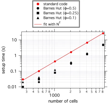
We have conducted calculations with the Barnes-Hut and standard methods using the plane strain stiffness coefficients with periodic boundary conditions (4). As mentioned pre-viously, the construction of the complete Kij matrix
con-sists of calculatingN2coefficients. This is setup time prior to the actual time-stepping calculation of displacement and stress. The setup time in our implementation of the stan-dard method reflects the expectedN2 scaling (Fig. 4). The overhead associated with setting up the smaller K matrix for the Barnes-Hut method is in practice about ten times shorter than for the standard calculation (Fig. 4). So, there is less overhead associated with the Barnes-Hut method, despite it having a somewhat complicated tree structure.
Fig. 4. Scaling of set-up time for boundary element calculations with the number of cells (N) used in the calculation. This plot shows how the observed time necessary to construct the stiffness matrix (e.g., Eq. 1), (setup time) increases with the number of cells
N. Red symbols are for the standard implementation. The red line has a slope of 2 corresponding to scaling ofN2. The black sym-bols define the scaling of setup for the BHM. The absolute setup duration is smaller for the BHM than for the standard approach.
as NlogN as expected (Fig. 5). For 4096 elements the BHM is more than 10 times faster and for 16 384 elements more than 30 times faster.
4 Example faulting calculations with the Barnes-Hut method
For this method to be useful in large scale faulting calcu-lations requires it to adequately reproduce the elastic inter-actions that it approximates. We illustrate the method in two different faulting applications: earthquake nucleation and pe-riodic rupture of an asperity. Our interest in this paper is to document that the BHM produces reliable approximations and to quantifying the associated errors.
4.1 Nucleation
Up until recently, earthquake nucleation as inferred from lab-oratory experiments was thought result from slip increasing monotonically within a patch of constant size, the size being determined by the asperity contact dimension, elastic proper-ties, and the dependence of the fault strength on slip rate. Di-rect observations of nucleation (Okubo and Dieterich, 1981, 1984), and some plane strain simulations (Dieterich, 1992)
Fig. 5. Scaling of execution time with number of elements for nu-cleation with the Barnes-Hut scheme forφ= 0.5 (black symbols), and with the standard method (red symbols) for 100 time steps. Shown for comparisons are lines followingN2andNlogNscaling.
support this simple view. The Dieterich (1992) simulations use the particular constitutive relations for friction
τ=σef=σe
fo+aln V V0
+blnV0θ
dc
(5a)
dθ dt =1−
θ V dc
(5b) (Ruina, 1983). Hereσe is the effective normal stress,f is the ratio of shear to normal stress, V is slip velocity, and
θ is a state-variable, which allows the fault to strengthen at very low sliding rates. The state variable has a steady-state valuedc/V0. V0andf0are reference values of velocity and friction, respectively, anddcis a characteristic displacement associated with changes in shear resistance during sliding.
Due to the complicated non-linear friction equations and spatial variations in slip, faulting simulations using (5a) and (5b) are necessarily done numerically. In Dieterich’s (1992) numerical calculations the resulting nucleation patch size is constant. Extrapolations to natural stressing rates using lab-oratory measured parameters suggest that it would be im-possible to resolve nucleation using surface and space-based strain sensors, and would be extremely difficult to detect in the subsurface using the most sophisticated borehole strain meters (Dieterich, 1992).
(a)
(b)
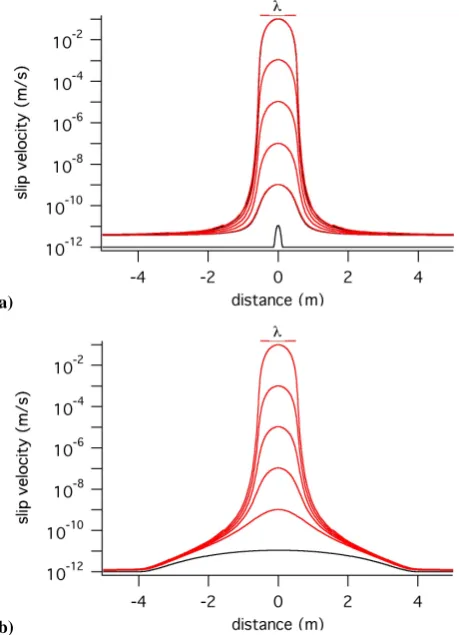
Fig. 6. Rupture initiation using slip and slip rate dependent fault strength (5a) and (5c) and the Barnes-Hut scheme withφ= 0.5 on a plane strain fault grid of 40 m length and periodic boundary condi-tions. In these calculationsf0= 0.7a= 0.008,b= 0.012,dc= 1 µm,
σn= 6 MPaτ= 0,G= 2.1×10⁴MPa, andν= 0.25. (a) Initial slip rate (black) is uniform atVs= 1×10⁻¹²m/s outside a centered per-turbation of 0.25 m width. The form of the perper-turbation is one half of 0.5 m wave length cosine function of peak to peak amplitude 10·Vstart. Different curves show increasing slip velocity within the patch with time. The solution without the Barnes-Hut approxima-tion is also shown but differences between it and BH are not really visible at this scale. Shown for reference is the dominant wave-length as inferred by Dieterich (1992). (b) Same as in (a) except the width of the perturbation (black) is 8 m.
(5b) approaches 1. For this previously unrecognized regime, nucleation patch sizes can be orders of magnitude larger. Were this behavior general, nucleation might be easier to detect in the earth, and, in general, departures from fixed patch length nucleation cast some doubts on what we think we know about earthquake occurrence from lab studies (Di-eterich, 1986, 1992).
During nucleation the state evolution relation can be sim-plified from the slip, time and slip rate dependent (5b) to an approximate form
dθ dt = −
θ V dc
, (5c)
(Dieterich, 1992) which is exponential in slip. To illus-trate the BHM in a first example we simulate earthquake nu-cleation using the slip and slip rate dependent relation for friction that results from combining (5a) and (5c)
τ=σe
f0+aln V
V0
−bδ
dc
. (5d)
We assume the slip velocity is initially uniform at velocity
Vstartexcept in a small region in the center of the grid where velocity is perturbed by a sinusoid of amplitude 10·Vstart (Fig. 6).
During nucleation (5b) has a stable characteristic nucle-ation patch size (see Dieterich, 1992; Rubin and Ampuero, 2005) for ratios of a/b <0.5, and expanding, crack-like behavior fora/b >0.5. Instead, for (6), our calculation with
a/b= 0.66 (Fig. 6) shows growth of a fixed length patch and generally we find that fixed length nucleation occurs for (5c) at all values ofa/b. Though Rubin and Ampuero (2005) did not consider the behavior of (5c), our observation of a fixed length patch is expected based on their results. Par-ticularly, they find that healing is not important for (5b) for low values of a/b. This lack of healing leads to the fixed length patch. Since (5c) is (5b) with the healing term re-moved, our result can be easily reconciled with Rubin and Ampuero (2005). The time dependent calculations carried out for this study show identical lengths for patches grow-ing from perturbations longer and shorter than the final patch length (Fig. 6) and that wavelength is as inferred by (Di-eterich, 1992) λ= 3.4Gdc/bσn. Shown for comparison in
Fig. 6a are the solutions without the BH approximation. These are in black beneath the BH solutions and are difficult to see at this scale; the BH approximation is a satisfactory representation of the solution over the entire grid.
4.1.1 Errors
For this range ofφthe maximum errors in slip range from 0.3% to 25% and average errors range from 0.06% to 4%. To achieve maximum errors of 1% or better,φ <0.2 is required. To begin to understand the errors in the solution and how they vary withφ, first consider errors associated with replac-ing external cells with a parent; these indicate how well dis-tant forces are approximated. Ignoring contributions from the replicates, (4) can be rewritten as
Kij= G
2π (1−υ)
1
Xij
− 1
Xij−1
≈ G
2π (1−υ)
Dx
X2ij
!
, (6)
and we see that the influence coefficients increase in propor-tion to the cell size Dx. Recall that Dx is a multiplen of the external cell size dx. When an external (child) cell is represented as part of a larger internal (parent) cell, stresses due to slip on that external cell will be represented by 1/n
of the stiffness coefficient of the internal cellKparent. In the full problem this same slip would be represented byKchild. The associated fractional error in the calculated stress due to using the internal cell instead of the external cell is
EK=
1−Kparent
nKchild
. (7)
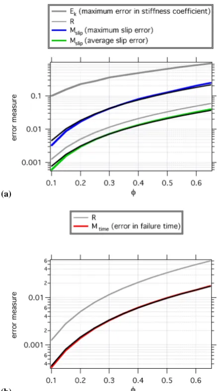
The actual maximum errors associated with the influence co-efficients as calculated from (7) are shown in Fig. 7a. These errorsEKforφ= 0.1 to 0.65 (thick grey line) are large,
rang-ing from 10% to 1% (Fig. 7a). They are much larger than the actual maximum errors in slip observed in the calculation (blue, Fig. 7a), and are still larger than the average errors in slip (green, Fig. 7a). The reason for the difference between the errors in stiffness and in slip is that the actual errors in slip result only in part from the error explicitly associated with the approximation. The further error reduction results because Kij for the nearest cells are not approximated and
the nearest cells have the have the largest influence. Thus, Eq. (7) represents an upper and unrealized bound on the er-rors in this BHM.
To get a better idea of the source of error in the BH ap-proximation, consider the absolute value of the ratio of the maximum parent influence coefficient to the maximum influ-ence coefficient. As described in the appendix, this ratio,R, can be calculated analytically for our uniformly spaced grid,
R= 1
81
φ2−
1 4
. (8)
R is a small number ranging between 0.001 and 0.06 asφ
increases from 0.1 to 0.65 (Fig. 7a). The ratio signifies that the distant and approximate influence coefficients are small relative to the nearby exact coefficients. This explains qual-itatively why the maximum error in the stiffness coefficients
Ekgreatly over-estimates the observed errors. For this
nucle-ation problem Eq. (8) shows nearly the same varinucle-ation with
φas the maximum and average slip. Empirically we can use
(a)
(b)
Fig. 7. Errors in the BHM for nucleation using the Barnes-Hut scheme asφis varied between 0.1 and 0.65. (a) Errors associated with the stiffness coefficients (Ek, Eq. 7 thick grey line) and with fault slip (M, blue and green). TheMare from the numerical sim-ulations. Shown also isR (Eq. 8, grey) which is the ratio of the maximum parent stiffness coefficient to the maximum stiffness co-efficient. The black curves are fits of the form ofRto the observed maximum and average errors in slip. These correspond to 3.6Rand 0.62R. (b). Errors associated with time of failure (M, red). These are from the numerical simulations. Shown also isR(Eq. 8, grey). The black curve is a fit of the form ofRto the observed failure time error.
3.6Ras an estimate of the maximum error in slip and 0.62R
for the average error. These estimates of the errors are the black curves in Fig. 7a. To insure an error of 1% in slip re-quiresφ <0.2.
are done with a modest number of segments (N= 2048) and the fractional increase in execution time of the BHM, the speedup, should scale asN/logN, we expect more significant time savings for larger scale simulations. 1% error on failure time can be achieved even withφ= 0.5 (Fig. 7b). Estimates of failure time can be efficiently calculated, preserving the overall behavior despite being approximate in detail. Again,
R(8) shows nearly the same variation withφis failure time. Empirically we can use 0.29Ras an estimate of the error in failure time. This error estimate is shown as the black line in Fig. 7b.
4.2 Periodic asperity failure
High-resolution seismological studies of creeping faults have revealed small repeating earthquakes with short recurrence intervals (typicallytr<5 yrs). These repeating earthquakes occur on different faults and in different tectonic settings, for instance on the Calaveras fault in the aftershock zone of 1984
M6.1 Morgan Hill, California earthquake (Vidale et al., 1994), within the aftershocks of the 1989M6.9 Loma Pri-eta, California earthquake (Schaff et al., 1998), on the Park-field, California segment of the San Andreas fault (Nadeau and Johnson, 1998) where one such event is the target of the SAFOD project, on the Hayward fault in Northern Califor-nia (Burgmann et al., 2000) and in subduction zones (Mat-suzawa et al., 2002; Uchida et al., 2005). Failure is thought to occur on a single asperity or fault patch embedded in an aseismically creeping fault plane (Vidale et al., 1994; Ellsworth, 1995; Nadeau and Johnson, 1998; Nadeau and McEvilly, 1999). In this case, recurrence is influenced by the rate of aseismic creep of the fault surrounding the patch, as geodetically measured fault creep correlates with cumu-lative earthquake moment release rate and with recurrence interval (e.g., Ellsworth, 1995). Study of small earthquakes with short recurrence may provide insight into the behavior of larger repeating earthquakes that are of greater interest be-cause of their greater damage potential, but are more difficult to study because they have much longer recurrence. On the other hand, small repeating earthquakes may be controlled by different fault physics due to their small slip and lower fric-tional heating. In that case source parameters and recurrence statistics of small repeating earthquakes may not be directly related to the large and hazardous events.
Our second example for testing the Barnes-Hut approx-imation is periodic failure of a small earthquake embed-ded on an otherwise aseismically creeping fault plane. The geometry is similar to 3D simulations by Chen and La-pusta (2009), but our calculations are plane strain and fully quasi-static while Chen and Lapusta (2009) use fully elasto-dynamic equations during rupture propagation. We simulate periodic asperity failure using Eqs. (5a) and (5b). The fault is loaded by an imposed constant slip rateVplateat the ends of the grid. The asperity has a<b, whereas outside the asperity
b= 0. This configuration results in continuous aseismic slip
of the fault well outside the asperity and stick-slip within the asperity. To account for radiated energy resulting from rapid slip we use the radiation damping approach of Rice (1993). Accordingly, stress change due to slip at each segmentiis
1τi=
X
j
Kijδj−η dδi
dt (9)
where the effective shear impedanceη=µ
2β, andµandβ
are the shear modulus and wave speed, respectively.
For a 10 m patch in the center of a 1000 m long fault with
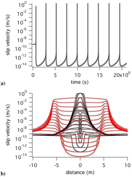
Vplate= 7.927×10⁻¹⁰m/s, the fault slips periodically with recurrencetr= 27.9 days (Fig. 8a). The space/time history of slip in the region containing the patch is well approximated with the BH approximation over the entire grid (Fig. 8b). Nucleation is different from the fixed width nucleation case (Fig. 6). Loading at the asperity edges leads to creep near the inner edge of the patch at nearly the same rate as outside the patch. Nucleation proceeds initially as the higher slip rate eats in towards the center from the edges. Over time the cen-ter of the patch accelerates. The region of accelerating slip is initially nearly the full asperity dimension but narrows with time. In the last stages of nucleation the patch length is simi-lar in width to that in the simple nucleation example. Despite the patch being loaded directly at the patch edge, nucleation of rupture ultimately occurs at the patch center and rupture propagates outward bilaterally to the edges. Rapid slip ex-tends outside the patch into the rate strengthening surround-ings. In these calculations, deceleration and arrest proceeds preferentially in the patch center while the edges continue to creep at an appreciable rate. This creep at the edges is essen-tially the early stages of afterslip in the surroundings. Note that aspects of propagation and arrest in nature may be influ-enced by elastodynamics not included in these calculations. 4.2.1 Errors
We calculated the errors forφ= 0.1 to 0.65 using 8192 cells. To examine errors, as in the nucleation case, we stop the sim-ulation when the slip velocity reaches 1 mm/s. In this imple-mentation slip is not calculated so we determine the maxi-mum errors in stress (Fig. 9) which range from 0.8% to 18%. The errors in stress are not as systematic as the errors in slip in the nucleation example. To achieve maximum errors of 1% or better errors,φ <0.2 is required. As in the nucleation example, the actual maximum errors associated with the in-fluence coefficientsEk as calculated from (7) are shown for reference (Fig. 9, thick grey line) and they are larger than the actual maximum errors in stress observed in the calculation. Shown also for reference is the ratioR. As in the nucleation exampleEk andR bound the errors in stress. Failure time
(a)
(b)
Fig. 8. Simulation of repeated slip of a seismic asperity embed-ded in an otherwise aseismically creeping fault. Equations (5a) and (5b) are used in the Barnes-Hut scheme on a plane strain fault grid of 1000 m length. The asperity is 10 m long. The calcula-tion approximates periodic boundary condicalcula-tions at the fault ends, that is, the fault is repeated along strike in both directions. For a true periodic boundary, the fault is repeated infinitely in both di-rections; in this calculation there are 1000 repeats of the fault in each direction The fault is loaded at both ends at constant rate
Vplate= 7.927×10⁻¹⁰m/s. a= 0.008, dc= 10 µm, σn= 60 MPa
τ= 0,G= 2.1×10⁴MPa,β= 3 km/s, andν= 0.25. Inside the patch
f0= 0.7 andb= 0.012, outside the patchf0= 0.2 andb= 0.0. (a) Time history of slip velocity on the element in the center of the patch from the BH approximate (φ= 0.1, black) and the standard solution (φ= 0.0, grey). The slight differences are difficult to see at this scale. The recurrence is characteristic with period∼27.9 days. (b) Time-space evolution of slip rate about the patch during a single recurrence. Contours are spaced by changes of an order of mag-nitude at the center element. Forφ= 0.1, black curves denote be-haviour during nucleation, the lower most black curve corresponds to the initial stages of nucleation. Forφ= 0.1, the red curves show the stages of rupture arrest and afterslip. Also shown in grey are the corresponding solutions forφ= 0.0.
the speedup, scales asN/logN, and we expect more signif-icant time savings for larger scale simulations. 1% error on failure time can be achieved even withφ= 0. 5 (Fig. 7b). Again as with the nucleation example, results can be calcu-lated efficiently that preserve the overall behavior despite be-ing approximate in detail.
Fig. 9. Errors in the BHM for repeated slip of an asperity asφis varied between 0.1 and 0.6. Equations (5a) and (5b) are used in the Barnes-Hut scheme on a plane strain fault grid of 40 m length. The asperity is 10 m long. The errors associated with the stiffness coef-ficients (Ek, Eq. 7 thick grey line), with shear stress (M, blue) and with failure time (M, red) are shown. These are from the numerical simulations. Shown also isR(Eq. 8, grey).
5 Conclusions/future work
Our interest in the Barnes-Hut method is to improve compu-tational efficiency for developing “earthquake simulators”. The simulators use natural fault network geometries, long-term slip rates and recurrence data along with particular as-sumptions about source physics and friction to produce syn-thetic seismicity catalogs. The objective of the simulators is to reproduce the overall statistical properties of earth-quakes, e.g., frequency magnitude relations, interevent times or aftershock-foreshock statistics associated with particular synthetic earthquakes on specific faults within an extensive model of a natural fault system.
simulator as our objective was to demonstrate the efficiency of the method and document the associated errors. Regard-less, we expect the method can be used to calculate elastic interactions on irregular grid sizes, for 2- and 3-D faults, and with complicated boundary conditions.
Subsequent to Barnes and Hut’s (1986) study, more so-phisticated approximate algorithms have been developed, no-tably the fast multipole method (Greengard and Rokhlin, 1987) in which the order of error is explicitly specified in the method, rather than indirectly determined from numeri-cal experimentation. In principle the fast multipole method is capable of scaling asN, rather thanNlogN. Prior to our study, a method for calculating fault slip based on Warren and Salmon (1993, 1994) has been developed by Tullis et al. (1999, 2000, 2004). Though this method has been referred to as a FMM, the number of interactions scales asNlogN, rather than asN. To date there are no peer-reviewed publica-tions of this approach.
We expect that improvements in performance of the FFM in faulting calculations are imminent; a fast multipole imple-mentation for faulting using dislocation segments is under development as an extension of the present study and inde-pendently by Tullis et al. On the other hand, in addition to the immense savings in computation time over standard method-ology, in existing codes that use dislocation solutions (e.g., Chinnery, 1963; Okada, 1985, 1992) the Barnes-Hut method is much easier to program and implement than fast multipole approaches. A BHM earthquake simulator code is also under development as an extension of the present study.
Appendix A
Here we estimate R, the absolute value of the ratio of the largest parent stiffness coefficient to the largest stiffness co-efficient. This ratio gives some indication of how important the contributions from the internal segments are relative to the external segments. For this estimate we ignore the con-tributions from the replicates in (4)
Kij= G
2π (1−υ)
1
Xij
− 1
Xij−1
. (A1)
(A1) is the plane strain solution lacking the periodic bound-aries (Weertman, 1979; Dieterich, 1992). Recall thatXij and
Xij−1are the distances between the center of the target seg-ment (external segseg-ment) and the right and left edges of the source segment (internal segment) (Fig. 3),Xij−1=Xij–Dx.
Again, noting that Dx is the width of the source cell, (A1) can be rewritten as
Kij= G
2π (1−υ)
Dx
Xij Xij+Dx !
. (A2)
Using the criteria for lumping the elements, we consider the minimum distance between the source (external segment) and the target (internal segment) for the source to be included
in the calculation, defined byL= Dx/φ. Also noting thatL
is measured between the element centers and is so defined as
L=Xij+Dx/2 and making both these substitutions into (A2) we find
Kij = G
2π (1−υ)
Dx
Dx
φ −
Dx 2
2
+DxDxφ −Dx
2
= G
2π (1−υ)Dx1
φ2−
1 4
. (A3) We use this expression (A3) for the parent stiffness coeffi-cient. The largest influence coefficient is due to self-slip of the target segment. (A1) for this target slip is
Kij= − G
2π (1−υ)
2 dx+
2 dx
= − 2G
π (1−υ)dx. (A4)
Ris the absolute value of the ratio of (A3) to (A4) or
R= dx
4Dx1
φ2−
1 4
. (A5) Recalling that the internal segment length Dx is a multiple of the external length dx, (A5) is at its maximum when Dx=2dx and we find the maximum to be
R= 1
81
φ2−
1 4
. (A6)
Acknowledgements. This study was supported by Southern
California Earthquake Center and NASA Earth Science program through grants to Terry Tullis of Brown University, and by the US Geological Survey Venture Capital Fund. Calculations used USGS and NASA computing facilities with technical advice and program-ming assistance from Larry Baker (USGS/EHZ) and Art Lanzanoff (NASA Ames). Thanks to Andrea Donnellean of NASA/JPL for support. This study followed from a collaboration by the authors with John Salmon. The wavenumber domain plane strain program used to verify errors in the BH solutions was written by Allan Rubin. Conversations with Allan provided insights on nucleation and recurrence that informed the example simulations. This paper was greatly improved in response to reviews by Ruth Harris, Steve Schilling, Mike Poland, Brad Aagaard, Keith Richards-Dinger, Gregor Hillers and the NPG editor Bruce Malamud.
Edited by: B. Malamud
Reviewed by: K. Richards-Dinger, G. Hillers, and two anonymous referees
References
Barnes, J. and Hut, P.: A Hierarchical O(N log N) force calculation algorithm, Nature, 324, 446 pp., 1986.
Ben-Zion, Y. and Rice, J. R.: Earthquake failure sequences along a cellular fault zone in a three-dimensional elastic solid containing asperity and nonasperity regions, J. Geophys. Res., 98, 14109– 14131, 1993.
Ben-Zion, Y. and Rice, J. R.: Slip patterns and earthquake popula-tions along different classes of faults in elastic solids, J. Geophys. Res., 100, 12959–12983, 1995.
Ben-Zion, Y.: Collective behavior of earthquakes and faults: Continuum-discrete transitions, progressive evolutionary changes, and different dynamic regimes, Rev. Geophys., 46, RG4006, doi:10.1029/2008RG000260, 2008.
Brune, J. N.: Tectonic stress and the spectra of seismic shear waves from earthquakes, J. Geophys. Res., 75, 4997–5009, 1970. Burgmann, R., Schmidt, D., Nadeau, R. M., d’Alessio, M.,
Field-ing, E., Manaker, D., McEvilly, T. V., and Murray, M. H.: Earth-quake potential along the Northern Hayward Fault, California, Science, 2000.
Burridge, R. and Knopoff, L.: Model and theoretical seismicity, B. Seismol. Soc. Am., 57, 341–371, 1967.
Carlson, J. M. and Langer, J. S.: Mechanical model of an earthquake fault, Phys. Rev. A, 40, 6470–6484, 1989a.
Carlson, J. M. and Langer, J. S.: Properties of earthquakes gener-ated by fault dynamics, Phys. Rev. Lett., 62, 2632–2635, 1989b. Cayol, V., Dieterich, J. H., Okamura, A. T., and Miklius, A.: High magma storage rates before the 1983 eruption of Kilauea, Hawaii, Science, 288, 2343–2346, 2000.
Chinnery, M. A.: The stress changes that accompany strike-slip faulting, B. Seismol. Soc. Am., 53, 921–932, 1963.
Das, S. and Scholz C. H.: Theory of time-dependent rupture in the Earth, J. Geophys. Res., 86, 6039–6051, 1981.
Dieterich, J. H.: Time-dependent friction in rocks, J. Geophys. Res., 77, 3690–3697, 1972.
Dieterich, J. H.: Modeling of rock friction, 1. Experimental results and constitutive equations, J. Geophys. Res., 84, 2161–2168, 1979.
Dieterich, J. H.: A model for the nucleation of earthquake slip, in: Earthquake Source mechanics, edited by: Das, S., Boatwright, J., and Scholz, C. H., Geophys Monograph 6, 37–47, 1986. Dieterich, J. H.: Earthquake nucleation on faults with rate- and
state-dependent strength, Tectonophysics, 211, 115–134, 1992. Dieterich, J. H.: A constitutive law for rate of earthquake production
and its application to earthquake clustering, J. Geophys. Res., 99, 2601–2618, 1994.
Dieterich, J. H.: Earthquake simulations with time-dependent nu-cleation and long-range interactions, Nonlin. Processes Geo-phys., 2, 109–120, doi:10.5194/npg-2-109-1995, 1995.
Dieterich, J. H. and Richards-Dinger, K. B.: Earthquake recur-rence in simulated fault systems, Pure Appl. Geophys., 167(8–9), 1087–1104, doi:10.1007/s00024-010-0094-0, 2010.
Ellsworth, W. L.: Characteristic earthquakes and long-term earth-quake forecasts: Implications of central California seismicity, in: Urban disaster mitigation: the role of science and technology, edited by: Cheng, F. Y. and Sheu, M. S., Elsevier, 1–14, 1995. Greengard, L. and Rokhlin, V.: A fast algorithm for particle
simu-lation, J. Comp. Phys., 73, 325–348, 1987.
Hirata, T.: Omori’s power law aftershock sequences of microfrac-turing in rock fracture experiment, J. Geophys. Res., 92, 6215–
6221, 1987.
Knopoff, L.: Model of aftershock occurrence, in: Flow and fracture of rocks, Geophys. Monograph, 16, 259–263, 1972.
Kranz, R. L.: The effects of confining pressure and stress difference on static fatigue of granite, J. Geophys. Res., 85(B4), 1854–1866, 1980.
Marcellini, A.: Arrhenius behavior of aftershock sequences, J. Geo-phys. Res., 100, 6463–6468, 1995.
Marcellini, A.: Physical model of aftershock temporal behavior, Tectonophysics, 277, 137–146, 1997.
Matsuzawa, T., Igarashi, T., and Hasegawa, A.: Characteristic small earthquake sequence off Sanriku, northeastern Honshu, Japan, Geophys. Res. Lett., 29(11), 1543, doi:10.1029/2001GL014632, 2002.
Mogi, K.: Study of elastic shocks caused by the fracture of hetero-geneous materials and their relation to earthquake phenomenon, B. Earthq. Res. Inst. Univ. Tokyo, Japan, 40, 125–173, 1962. Nadeau, R. M. and Johnson, L. R.: Seismological studies at
Park-field VI: Moment release rates and estimates of source parame-ters for small repeating earthquakes, B. Seismol. Soc. Am., 88, 790–814, 1998.
Nadeau, R. M. and McEvilly, T. V.: Fault slip rates at depth from re-currence intervals of repeating microearthquakes, Science, 285, 718–721, 1999.
Okada, Y.: Surface deformation due to shear and tensile faults in an half-space, B. Seismol. Soc. Am., 75(4), 1135–1154, 1985. Okada, Y.: Internal deformation due to shear and tensile faults in an
half-space, B. Seismol. Soc. Am., 82(2), 1018–1040, 1992. Okubo, P. G. and Dieterich, J. H.: Fracture energy of stick-slip
events in a large scale biaxial experiment, Geophys. Res. Lett., 8, 887–890, 1981.
Okubo, P. G. and Dieterich, J. H.: Effects of physical fault prop-erties on frictional instabilities produced on simulated faults, J. Geophys. Res., 89, 5817–5827, 1984.
Rice, J. R.: Spatio-temporal complexity of slip on a fault, J. Geo-phys. Res., 98, 9885 – 9907, 1993.
Robinson, R. and Benites, R.: Synthetic seismicity models of multi-ple interacting faults, J. Geophys. Res., 100, 18229–18238, 1995. Robinson, R. and Benites, R.: Synthetic seismicity models for the Wellington region, New Zealand: Implications for the temporal distribution of large events, J. Geophys. Res., 101, 27833–27844, 1996.
Rubin, A. M. and Ampuero, J.-P.: Earthquake nucleation on (aging) rate-and-state faults, J. Geophys. Res., 110, B11312, doi:10.1029/2005JB003686, 2005.
Reuschle, T. Slow crack growth and aftershock sequences, Geo-phys. Res. Lett., 17, 1525–1528, 1990.
Rundle, J. B.: A physical model for earthquakes, 1. Fluctuations and interactions, J. Geophys. Res., 93, 6237–6254, 1988a. Rundle, J. B.: A physical model for earthquakes, 2: Application to
Southern California, J. Geophys. Res., 93, 6255–6274, 1988b. Ruina, A. L.: Slip instability and state variable friction laws, J.
Geo-phys. Res., 88, 10359–10370, 1983.
Schaff, D. P, Beroza, G. C., and Shaw, B. E.: Postseismic response of repeating aftershocks, Geophys Res. Lett., 25, 4559–4552, 1999.
Scholz, C. H.: Mechanism of creep in brittle rock, J. Geophys. Res., 73, 3295–3302, 1968a.
Soc. Am., 58, 117–130, 1968b.
Scholz, C. H.: Static fatigue in quartz, J. Geophys. Res., 77, 2104– 2114, 1972.
Stein, R. S., Barka, A. A., and Dieterich, J. H.: Progressive fail-ure on the North Anatolian fault since 1939 by earthquake stress triggering, Geophys. J. Int., 128, 594–604, 1997.
Tullis, T. E., Salmon, J., Kato, N., and Warren, M.: The application of fast multipole methods to increase the efficiency of a single-fault numerical earthquake model, EOS T. Am. Geophys. Un., Fall Meeting Suppl., 80, F924, 1999.
Tullis, T. E., Salmon, J., and Kato, N.: Use of fast multipoles for earthquake modeling, Proceedings of Second ACES Workshop, Tokyo and Hakone, Japan, 15–20 October 2000, 35–40, 2000. Tullis, T. E., Noda, H., Richards-Dinger, K., Lapusta, N., Dieterich,
J. H., Kaneko, Y., and Beeler, N. M.: Comparing Earthquake Simulators That Include Rate and State Friction, EOS T. Am. Geophys. Un., Fall Meet. Suppl., 90(52), Abstract T21B-1807, 2009.
Tullis, T. E.: Detailed multi-scale earthquake modeling using rate and state friction and the fast multipole method on parallel com-puters, EOS T. Am. Geophys. Un., Fall Meeting Suppl., 85(47), NG54A-06, 2004.
Turcotte, D. L. and Schubert, G.: Geodynamics applications of con-tinuum physics to geological problems, John Wiley and Sons, 450 pp., 1982.
Uchida, N., Matsuzawa, T., Hasegawa, A., and Igarashi, T.: Recur-rence intervals of characteristic M4.8+/–0.1 earthquakes off Ka-maishi, NE Japan, Comparison with creep rate estimated from small repeating earthquake data, Earth Planet. Sci. Lett., 233, 155–165, 2005.
Vidale, J. E., Ellsworth, W. L., Cole, A., and Marone, C.: Rupture variation with recurrence interval in 18 cycles of a small earth-quake, Nature, 368, 624–626, 1994.
Ward, S. N.: An application of synthetic seismicity calculations in earthquake statistics: The middle American trench, J. Geophys. Res., 97, 6675–6682, 2000.
Ward, S. N.: San Francisco Bay Area Earthquake Simulations: A step toward a Standard Physical Earthquake Model, B. Seismol. Soc. Am., 90, 370–386, 2000.
Warren, M. S. and Salmon, J. K.: A parallel hashed Oct-Tree N-body algorithm, in: Supercomputing ’93, Proceedings of the 1993 ACM/IEEE conference on Supercomputing, Portland, Ore-gon, USA, ACM, New York, NY, USA, 12–21, ISBN:0-8186-4340-4, 1993.
Warren, M. S. and Salmon, J. K.: A fast tree code for many-body problems, in: Los Alamos Science, edited by: Cooper, N. G., Los Alamos National Laboratory, Los Alamos, NM, 22, 88–97, 1994.
Weertman, J.: Inherent instability of quasi-static creep slippage on a fault, J. Geophys. Res., 84, 2146–2152, 1979.
Working Group on California Earthquake Probabilities (WGCEP): Earthquake probabilities in the San Francisco Bay region: 2002 to 2031, US Geol. Surv. Open-File Report No. 03-214, 2003. Working Group on California Earthquake Probabilities (WGCEP):
The uniform California earthquake rupture forecast, Version 2 (UCERF 2), 2007.