Assessment of sensor performance

(1)

www.ocean-sci.net/6/235/2010/

Ocean Science

Assessment of sensor performance

C. Waldmann1, M. Tamburri2, R. D. Prien3, and P. Fietzek4 1_{Bremen University/MARUM, Bremen, Germany}

2_{Alliance for Coastal Technologies, University of Maryland Center for Environmental Science, USA} 3_{Leibniz Institute for Baltic Sea Research, Warnemuende, Germany}

4_{IFM-GEOMAR, Kiel, Germany}

Received: 8 June 2009 – Published in Ocean Sci. Discuss.: 31 July 2009

Revised: 24 November 2009 – Accepted: 30 November 2009 – Published: 17 February 2010

Abstract. There is an international commitment to develop

a comprehensive, coordinated and sustained ocean observa-tion system. However, a foundaobserva-tion for any observing, mon-itoring or research effort is effective and reliable in situ sen-sor technologies that accurately measure key environmental parameters. Ultimately, the data used for modelling efforts, management decisions and rapid responses to ocean hazards are only as good as the instruments that collect them. There is also a compelling need to develop and incorporate new or novel technologies to improve all aspects of existing observ-ing systems and meet various emergobserv-ing challenges.

Assessment of Sensor Performance was a cross-cutting is-sues session at the international OceanSensors08 workshop in Warnem¨unde, Germany, which also has penetrated some of the papers published as a result of the workshop (Denu-ault, 2009; Kr¨oger et al., 2009; Zielinski et al., 2009). The discussions were focused on how best to classify and vali-date the instruments required for effective and reliable ocean observations and research. The following is a summary of the discussions and conclusions drawn from this workshop, which specifically addresses the characterisation of sensor systems, technology readiness levels, verification of sensor performance and quality management of sensor systems.

1 Introduction

Progress in any branch of science is heavily dependent on the types and required accuracy of measurements that are needed to describe the status and the processes under in-vestigation. In ocean sciences, physical and biogeochemical processes of diverse temporal and spatial scales are strongly

Correspondence to: C. Waldmann ([email protected])

coupled. Therefore, a huge variety of parameters is needed to uniquely characterise the status of the system and reveal the relationship between ongoing physical, chemical and biolog-ical processes. In this context, it is of the utmost importance to precisely state the level of knowledge with regard to mea-surement uncertainties for each of the relevant parameters being defined by the measuring principle and the respective instrument in use.

(2)

236 C. Waldmann et al.: Assessment of sensor performance it can lead to serious delays in efforts such as designing a

long-term monitoring strategy for the ocean environment on a global scale.

In the framework of the long-term ocean observations, such as the ARGO float program or the planned ocean obser-vatories, it is essential to reach consensus of assessment of the quality of the collected data (Pouliquen et al., 2009). The rationale for this is that the measured values are no longer just processed and used by an individual end-user or used for an individual mission, but they are made available for the entire ocean science community and perhaps for some measured values, perhaps well beyond the ocean science community, to the general public. Only if the end user has sufficient confi-dence in the quality of the collected data, and the information of different sources is directly comparable, will he or she be able to test models or use them for assimilation purposes.

Although appropriate services to help the end-user with issues such as calibration of instrumentation and measuring methodology are available, ocean sciences does not make full use of it. As a matter of fact, for certain parameters such as temperature and pressure, it is already common practice, but for almost all the other parameters it is not. The reason for that lies often in

– the lack of time/the need for quick results; in ocean

sci-ences, the focus is most often on the interpretation of data rather than on analysis of the measuring principle. Furthermore, as a consequence of the time pressure, ad-ditional services on instruments such as inspections or calibrations are avoided or reduced to a minimum, since these cause additional uncertainty with regard to their timely availability;

– cost considerations;

– the lack of knowledge;

– the lack of acceptance in the ocean science community;

– constraints imposed by the measuring method itself,

such as in the case of conductivity where laboratory cal-ibrations are very demanding (Saunders et al., 1991; Ba-con et al., 2007);

– alternative strategies employing extensive and complex

in situ intercomparisons of instruments employing the same measuring principle (Gouretski and Koltermann, 2007);

– the possibility of comparisons with other parameters

and judging on the accuracy based on consistency of the results (Bates et al., 2000).

These are not insurmountable obstacles. There simply has to be incentives to overcome the conventional attitude that the idea of building commonly used infrastructures might be a starting point. At the centre of the following discussion lies the description of a suggested basic vocabulary to describe

Table 1. Consolidation of TRL to OS-TRL.

Sensor development status

TRL Short description OS-TRL

Short description

1 Basic principles observed and reported

1 Proof-of-concept/development 2 Technology concept and/or

ap-plication formulated 3 Analytical and experimental

critical function and/or characteristic proof-of concept 4 Component and/or breadboard

validation in laboratory environment

2 Research Prototyping 5 Component and/or breadboard

validation in relevant environ-ment

6 System/subsystem model or prototype demonstration in a relevant environment 7 System prototype

demonstra-tion in a space/ocean environ-ment

3 Commercial product 8 Actual systems completed

and “ocean mission qualified” through test and demonstration 9 Actual system proven through

successful mission operations 4 Mission proved

the measurement process and the role and need of calibration and testing.

2 Definition of terms

In ocean sciences certain parameters that are measured have no unique definition in a metrological sense (e.g., primary productivity and turbidity). Rather, certain measuring rameters are used as an indirect measure (proxy) for the pa-rameter of interest. To preserve the pragmatic approach, at least the need to uniquely define the measuring process has to be satisfied to allow for the repetition of the measurement and/or by employing parameters measured in SI units to al-low for traceability.

(3)

The approach described above dictates that all branches of ocean sciences involved have a common vocabulary to uniquely describe the measurement process and constraints. Thus, the next necessary steps are to leverage existing knowl-edge about doing measurements which, for instance, in physics has been cultivated for centuries (Sullivan, 2001). The keepers of this knowledge are the national standard lab-oratories that are responsible for delivering and disseminat-ing calibration standards and methods in accordance with the definition of terms. It is part of their mission to support any activity that leads to an objective assessment of the perfor-mance of any kind of sensor system, be it in ocean sciences or any other branch.

As a first step towards achieving a unique assessment of sensor performance, a certain set of definitions and descrip-tion of terms becomes necessary. This can be summarised in a vocabulary, which is a terminological dictionary that con-tains designations and definitions from one or more specific subject fields. In this vocabulary, it is taken for granted that there is no fundamental difference in the basic principles of measurement in physics, chemistry, ocean sciences, biology or engineering. The International vocabulary of metrology – basic and general concepts and associated terms (VIM, 2007) is the reference for all national standard laboratories and should also be used for measurements in ocean sciences. As an example, a definition of the terms “resolution” and “sensitivity” is given in Appendix A1. These definitions clearly show how a careless use of terms can lead to con-fusion. In most cases, people are using the terms synony-mously, although they are mostly interested in the resolution of a measuring system to predict whether they could see a change in the parameter under investigation.

Another concept that comes into play and may help in the introduction of the illustrated principles is the Sensor Web Enablement (SWE/SensorML; M. Botts, University of Al-abama at Huntsville) concept that, besides other issues, aims at defining a so-called “controlled vocabulary to uniquely de-scribe sensor systems and the measuring process”. As SWE is following a process-oriented approach, which means that it only describes the process and gives references to definition of terms, VIM can be easily integrated. The ultimate goal of SWE is that, with the establishment and practical use, the end-user does not have to consider specific details of char-acterising the sensor in use, but can rather rely on the estab-lished metadata information system being delivered by the sensor itself through the entire processing chain. Currently there are still issues with the unique description of measure-ment properties with metadata. This goes back to the fact that every community is defining its own vocabulary in de-scribing the performance of their tools. The Marine Metadata Initiative (MMI project) is aiming to resolve some of the is-sues by, for example, offering tools to map vocabularies. In any case, a harmonised vocabulary or an according ontology is a necessary step to make ocean observation systems inter-operable.

In the past twenty years, a paradigm shift in measurement has occurred. In the classical approach (Kohlrausch, 1968), it has been assumed that the result of a measurement (the mea-surand) can be described by a single true value, and due to errors caused by the measuring instrument, the actual value is offset from the true value. The errors (i.e., the deviations from the true value) were typically designated as random and systematic errors. This led to the situation where no sin-gle value was attributed to a described measurement error, in large part because it was unclear how to treat these two separate numbers in a consistent way. The Guide on Uncer-tainty in Measurements (GUM, 2008) is addressing exactly this issue. It is much more helpful to introduce a single pa-rameter that can be calculated, and that papa-rameter is the un-certainty – . . . a parameter, associated with the result of a measurement that characterises the dispersion of the values that could reasonably be attributed to the measurand.

Within this new approach, the measuring process is judged as a system where the measurand, the measuring environ-ment and the measuring instruenviron-ment interact. This actual con-stellation leads to an uncertainty of the measurand. It used to be common practice to talk about measurement errors, while today, with the introduction of GUM, uncertainty is the ac-cepted term.

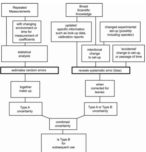
GUM replaces the formalism of random and systematic errors with Type A and Type B uncertainties. Type A eval-uations of uncertainty are based on the statistical analysis of a series of measurements. Type B evaluations of uncertainty are based on other sources of information such as an instru-ment manufacturer’s specifications, a calibration certificate, or values published in a data book. There are rules on how to combine Type A and B uncertainties into one quantity (see Fig. 1 and NIST 1994) depending on the actual measuring task. It should be noted that for subsequent use of the calcu-lated uncertainty, it has to be treated as Type B by agreement. A measurement result is expressed as a single measured quantity value and a measurement uncertainty:

Measured value = best estimate of value±uncertainty (1) where the best estimate could be, for example, the mean of a series of repeated measurements.

The uncertainty is calculated employing well-known sta-tistical methods evaluating the variance and standard devia-tion of the measurement sample. GUM recommends using the expanded uncertainty as the final number value, where the coverage probability or level of confidence of the speci-fied uncertainty is 95%. This is described with the coverage factork:

Uncertainty = k·standard deviation (2) If the probability should be 0.95 that all measured values are lying between±uncertainty of the best estimate, the cover-age factor,k, would be approximately equal to 2, depending on the type of the distribution law, e.g. Gaussian, Poisson etc.

(4)

238 C. Waldmann et al.: Assessment of sensor performance

– Internationally credited/accepted approach to

calculat-ing and expresscalculat-ing uncertainties.

– Allows everyone to “speak the same language”.

– Allows the term “uncertainty” to be interpreted in a

con-sistent manner.

– A “must” for everyone working in stan-dards/calibrations laboratories and growing in im-portance in industrial laboratories – key phrase is that it will “increase competitiveness”.

– Becoming essential knowledge in many other fields,

in-cluding forensic, medical and biomedical.

– Likely to be around for some time to come.

Until the advent of GUM, inconsistencies existed worldwide in the way uncertainties were calculated, combined and ex-pressed. Without international consensus on these matters, it is difficult to compare values obtained through measurement in different laboratories around the world.

SI units are often just seen as recommendations for speci-fying the units of measuring results. Obviously this is insuf-ficient, if measuring results are specified in SI units, as this also implies that the measurements are traceable to SI stan-dards. In fact, salinity, as it is defined in ocean sciences in 2009, is not traceable to SI units.

It is logical to make use of the competence that has been built up in national standard laboratories and independent, third-party test organizations. In order to become an integral part of the calibration chain defined by the national standard laboratories, which is also called metrological traceability, it is necessary to accept their procedures, policies and termi-nology. This would be the first step to achieve a consistent, coherent approach for ocean sciences. In cases where param-eters are not traceable to SI units, intermediate solutions have to be identified and established, as it is the case for salinity, which is related to an artefact namely to a potassium chlo-ride (KCl) solution containing a mass of 32.4356 grams of KCl. For each parameter, it has to be made clear how the measuring scale is defined, to what standards it refers to, and how the conducted measurement can be traced back to this standard.

In the appendix, a few definitions will be given for terms that are important to describe the performance of a sensor based on the International Vocabulary of Metrology (VIM), including notes with further descriptions.

3 Characterisation of sensor systems – generic sensor

model, identification of functional blocks

Sensor, transducer and detector – these terms are some-times used synonymously although they have slightly differ-ent meanings. In this text, a sensor shall be part of the trans-ducer, i.e. a transducer consists of a sensor plus signal con-ditioning circuitry, which is in compliance with VIM. Sensor and detector, for instance a photocell in a spectrophotometer, describe basically the same system and it depends on the type of measurement which term will be used. To define a sensor model that is in compliance with GUM, the basic measuring process has to be defined. A measurand or a parameterp un-der investigation often cannot be measured directly. There-fore, a number of input quantities have to be measured to determine the measuring value. This can be formally written as a functional relationship:

p=f (x1,x2,...,xn) (3)

wherex1. . .xn describe theninput quantities andpthe

pa-rameter of interest. The n input quantities can either be repeated measurements or different input parameters. The model allows for calculating the influence of the uncertainty in the individual input quantities xi on the measurement

valuep. Within a more generalised model, the step response time can be included in this model as well. Within GUM, this functional relationship (called the measurand model) is essential in determining the uncertainties taking all relevant input parameters into account.

As an example, the model of a platinum resistance ther-mometer is described through:

R(T )=R0(1+αT ) (4)

where R(T) is the resistance of the platinum element at the according temperatureT,R0is the resistance at 0◦C andα

is the temperature coefficient. Rearranging Eq. (3) to solve

T delivers:

T=R(T )−R0

R0α

(5) From this equation the Type B uncertainty for the tempera-ture,1T, can be calculated from:

1T= 1R

R0α

(6)

1T2=

1R R0α

2

+ 1R0·R

R₀2α

!2

+

1α·(R−R0)

α2_·_R 0

2

(7)

Where:

– 1Ris the uncertainty in the resistance measurement;

(5)

Fig. 1. The explanation and combination of Type A and Type B

uncertainties (from Kirkup et al., 2006). Type A uncertainties are related to the former random errors, while Type B uncertainties have a connection to the former systematic errors.

and in Eq. (6) it is assumed thatR0andαis exactly known

while in Eq. (7) the according errors are taken into account. The model is, therefore, a tool to calculate the propagation of uncertainties at the input through the different elements of the transducer system.

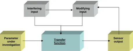
The block diagram of Fig. 2 shows a generic model of a sensor. The model function can be associated with the ex-tended transfer function of the sensor. This is of particular importance in calculating Type B uncertainties.

This schema should be considered as a start to identify cer-tain functional blocks of a generic sensor system, as cercer-tain aspects may still not be accounted for properly. For instance, a clear distinction between interfering input, which addresses added noise components and modifying input, which ac-counts for changes of the transfer function may not be possi-ble in all cases. In the figure, a feedback from the sensor out-put to the transfer function is inserted, accounting for possi-ble feedback mechanisms to correct for recurring/systematic errors.

It is obvious that for every sensor system and each appli-cation (e.g., ocean observatories), the schema or measurand model has to be stated and published. It is also important to clearly identify all possible measuring errors and to al-low the expert user to judge the performance of instruments. The final aim is to relieve potential users from this burden. A very good example where parts of these ideas have been implemented are acoustic Doppler current profiling

instru-ments. Although the measuring principle is rather straight-forward (frequency shifts are converted into current data), the actual processing steps are quite intricate. Accordingly the assessment of the data quality is only possible with ad-equate background knowledge. In any case, a formalization of the processing steps appears to be necessary, i.e. compre-hensive work flow descriptions and standard operating pro-cedures. Concepts like SWE can be an adequate framework for this process.

The aim of this exercise is to demonstrate that certain fea-tures are common to all sensor systems and, accordingly, that principles applying to one particular sensor system, for in-stance a CTD probe, may equally well be applied to other sensors (e.g., biochemical sensors). In the following para-graph, this concept is extended to the assessment of the de-velopment stage of a newly introduced sensor system.

4 Assessment of development status employing the

concept of Technology Readiness Level (TRL)

Sensors undergo different maturity levels during their de-velopment. From the time the method has been conceived through different realisation stages until final verification of the operational status through several successful missions, it is a process that may take several years or even decades. Al-though it is not uncommon for the development process to be extended in an attempt to produce a perfect instrument, technical constraints are often the most challenging and time consuming. If a prototype has been produced, the next obsta-cle is unforeseen effects derived, for instance, from ing parameters. In the case of an UV nitrate, sensor interfer-ences by higher concentrations of dissolved organic matter and carbonate, in particular in coastal and estuarine waters, are causing uncertainties.

Particularly in ocean sciences, the requirements on in situ measurements with regard to resolution and accuracy are ex-tremely high and often reach the limit of what can be done in the laboratory. In addition, the needs on the engineering side within ocean sciences are demanding as well. The discrep-ancy between the needs/expectations and limited time avail-able to finish product development can lead to unsatisfactory performance of new sensor systems. However, common ap-proaches of other science and engineering disciplines can be utilized to demonstrate what development steps are necessary until the final system is truly operational.

(6)

Transfer function Interfering

input

Sensor output Modifying

input

Parameter under investigation

Fig. 2. Generic sensor model or input-output schema, where

mod-ifying input means influencing the transfer function and interfering input means adding to the uncertainty as noise component.

for space technology planning (Mankins, 2005, see also Ap-pendix A2).

Obviously the TRL steps defined by NASA are very de-tailed in their description because this particular field has been using this type of scale for many years. In ocean sci-ences, this is certainly not the case. During the Ocean Sen-sors Workshop in Warnemuende, Germany (2008), it has been suggested to group individual TRL stages to consol-idated, four Ocean Sciences Technology Readiness Levels (OS-TRL):

1. Proof-of-concept/development (TRL 1–3); 2. Research prototyping (TRL 4–6);

3. Commercial (TRL 7–8); 4. Mission proved (TRL 9).

The transition from OS-TRL stage 3 to 4 should include in-dependent testing, validation and verification. The individual manufacturer or developer can classify their product into an appropriate TRL stage, but proof (adequate data and docu-mentation) must be made available. In contrast to the original TRLs, this schema assumes that all stages have to be passed in any case.

5 Verification of sensor performance and the role of cal-ibration procedures

A common problem in the development process is the veri-fication of the performance of a newly developed sensor by conducting laboratory calibrations, beta or field performance testing or in situ intercomparisons. It is not only necessary to demonstrate the operational status of the sensor itself, along with its manageability, but also the practicability of the rele-vant measurement method for a certain parameter under de-fined conditions. As mentioned, most parameters are con-nected to others by carrying implicit information about oth-ers. For example, electrical conductivity of seawater has a strong temperature dependence. Thus, conductivity values can be correlated with measured temperature profiles to iden-tify artefacts. Validation can be done in three different ways:

(1) Comparison with higher accuracy standard instruments or artefacts. Measurements are conducted in a calibra-tion laboratory with higher accuracy laboratory instru-ments or reference standards are sent around to differ-ent laboratories to perform intercomparisons. Both ap-proaches have their pros and cons, in particular, if oper-ational constraints are taken into account.

(2) Comparison with other methods measuring the same pa-rameter. This is of particular interest when performing in situ calibrations. Other methods can be based on wa-ter samples to be measured on the ship or alwa-ternative in situ sensors. As mentioned in the introduction, this also allows for verification of how precisely the mea-suring task or to-be-measured parameters have been de-fined in a physical sense. Vicarious calibrations also belong into that category where known events or phe-nomena are used to check for calibration shifts. For this to be successful, care has to be taken so that water with the same (or at least very similar) properties is sampled using the different methods.

(3) Comparison with another method measuring a parame-ter that carries implicit information about the parameparame-ter under investigation. This is combined with the use of a model that assimilates different parameters and finally leads to a statement in regard to the consistency of the individual parameters measured. This method can be described as a predictive model feedback. Again it has to be ascertained that the water sampled by the different methods has the same properties.

The independence of the validation or verification of a sen-sor is also critical for the credibility of results. An example for an independent and transparent type of third-party testing is the Technology Evaluations conducted by the Alliance for Coastal Technologies (ACT, http://www.act-us.info). ACT conducts two types of sensor testing. Technology Verifica-tions that equal TRL 7/8 or OS-TRL 3 are rigorous evalua-tions of commercially available instruments to verify man-ufacturers’ performance specifications or claims, which are carried out in the laboratory and under diverse field condi-tions and applicacondi-tions. Technology Demonstracondi-tions are a less extensive exercise where the abilities and potential of a new technology is established by working closely with develop-ers/manufacturers to field test instruments. This would cor-respond to TRL 6 or OS-TRL 2.

However, ACT only quantifies the performance of sensors against a community agreed standard (e.g., dissolved oxy-gen sensor against a Winkler titration) and not against other instruments.

(7)

certification of calibration facilities is not necessarily re-quired for the mentioned procedures. However, guidelines for assessing the sensor performance and the definition of standard operating procedures in testing and use of differ-ent sensor systems will be necessary in the future and should build up on existing efforts.

An often neglected fact is the dynamic behaviour of sen-sor systems. In many cases, the sensen-sor is not deployed at a single location for long-term measurements but is used for taking horizontal or vertical profiles. In the latter case, a well-defined dynamic model has to be used to correct or filter the raw data. The CTD gives a good example in that context, as temperature and conductivity sensor systems show com-pletely different temporal behaviour. Therefore, before the data are merged to derive salinity and density data, a dedi-cated filtering process is applied that matches the temporal behaviour of these sensors together. The metric to evaluate the quality of the result is the so-called spiking of the de-rived parameters that shows up in strong gradients. Again, it should be kept in mind that a lot of experience with the processing already exists in the realm of CTD, where, for instance, it has been shown that speeding up the sensor re-sponse by enhancing the higher frequency rere-sponse of the transfer function leads to extensive noise.

As most ocean measurements are done with multiple sen-sor systems, there are opportunities to examine the temporal performance of a newly designed sensor by comparison with other parameters to be collected. Strong gradients in temper-ature and salinity are often related to corresponding gradients in other parameters, which can then be used to validate the temporal performance of the sensor measuring the parameter of interest.

The users and manufacturers/developers of sensor systems are obviously two groups with distinct interests and within both groups problems regarding the quality of data can have their origin. While the user is interested in a flawless oper-ation without delving too deep into engineering issues, the manufacturer is often aware of limitations of the instrument that might result from the technical realisation of the sen-sor or is related to constraints based on basic physical prin-ciples. The communication process on these issues has to be improved. In this complex framework, standard labora-tories, and programs such as the Alliance for Coastal Tech-nologies (ACT), can play a role as a facilitator with regard to establishing a firm ground for assessing sensor performance. From their perspective, every process step, for instance with regard to calibration, has to be uniquely identified and made transparent to allow for control. This approach is strongly related to the concept of quality management. In the case of sensors, it means that every process step is clearly described and documented based on an agreed upon measuring proto-col or documentary standard. With the right guidelines, the calibration and testing of sensors can be conducted equally by companies or research institutions. Employing an accred-itation system, such as ISO/IEC 17025 (2005), each

manu-facturer would be able to specify its products according to agreed upon standards with appropriate documentation. The feasibility of this concept is demonstrated in everyday busi-ness all over the world.

This illustration also brings up the question whether a cen-tral ocean sensor calibration laboratory, either national or in-ternational, is needed. In particular, it has to be considered in the context that, within planned ocean observatories, hun-dreds of sensors shall be deployed and operated concurrently. Without attempting to answer the question conclusively, a distributed calibration system seems to be more viable and appropriate. To achieve comparability, consensus on testing and calibration procedures has to be reached. A promising example for a successful consensus on standard calibration and measuring techniques in the field of chemical oceanogra-phy without a laboratory entity being involved is reported in Dickson et al. (2007) and within the QUASIMEME project (QUASIMEME, 2009). This standard work in the field of ocean CO2 measurements incorporates contributions of

nu-merous scientists and was released under the auspices of PICES and UNESCO. A similar guide for ocean acidification research and data reporting is currently in review (Riebesell et al., 2009).

6 Quality management of sensor systems service and

maintenance procedures, implications for observato-ries

The need for instrument quality management is always es-sential and of particular importance when real-time data are collected and distributed. The users of these data should be able to retrieve all relevant information about sensor and re-sulting data quality either from the operator or another insti-tution that oversees the data collection process. In a quali-tative sense, it means that the data are made trustworthy by setting appropriate flags and, in a quantitative sense, that the uncertainty is specified.

Typically, quality management is associated with quality controls (QC), which in its simplest form means filtering out outliers. This is an unwanted but in most cases necessary step. In addition, there are also cases where this filtering process leads to significant errors, as natural variability can have an unexpected intensity. Therefore, the issue of QC is strongly interlinked between sensor performance and process evaluation. If one focuses on the sensor side, quality assur-ance is of utmost importassur-ance. That implies the following procedures:

– basic check of sensor by visual inspection and basic

electronic check;

– pre-deployment calibrations;

(8)

– monitoring the performance (temporal variability) at

sea;

– comparing with historical and climatological data;

– taking in situ water samples to compare with the sensor.

All the processing steps listed above have to be traceable by employing thorough documentation. Templates have been developed within certain laboratories in Europe (IFREMER, 2009) and North America (WHOI, 2009), and there is also a need to summarise the experience and to recommend best practices (Dickson, 2007). The impetus for that might again come from the different ocean observatory initiatives as has been described above. In any case, quality management pro-cedures are aiming to decentralise processes that lead to ac-curate ocean data and, therefore, they are of high importance in implementing a global data quality standard.

A number of initiatives in those directions already exist. There is the QARTOD/Q2O project funded by NOAA (see references on the QARTOD and Q2O projects) that is ex-plicitly addressing these issues and the Marine Metadata In-teroperability project (MMI project, 2009) coordinated by MBARI that aims at formalising the issues into interopera-ble metadata descriptions. These metadata will be accessiinteropera-ble and linked to the data streams.

7 Template sensor system – CTD as use case

Probably the best-known sensor system in ocean sciences is the CTD. Since the first laboratory tests 100 years ago (Forchhammer, 1865) and first in situ implementation in the 1950s (Hamon, 1958), CTDs have been extensively used and validated. Probably the most critical tests were with floats that had been in operation over several years, where drift was checked by employing well-knownT-Srelationships. With this approach, it has been demonstrated that, for instance, salinity drift in some CTD-system has been less than approx-imately 0.01 (units reported by instruments) after two years of operation (Janzen et al., 2008).

Calibration routines have been described in detail in dif-ferent publications, such as the UNESCO Technical Pa-pers (1994). In a sense, these works give a template of how to deal with other sensor systems, in particular, with regard to the description given for the CTD-sensors that involve in detail:

– modelling the sensor behaviour;

– definition of calibration routines, precautions in

opera-tion;

– processing of data;

– exchange of data.

All these are necessary steps to determine the operational status of a parameter in ocean sciences and assess the per-formance of the involved sensor system.

8 Conclusions and recommendations

Assessing sensor performance, and proper instrument cali-bration as well as use, is critical to the success of any ocean observing initiative, research program or management ef-fort. Instrument verification and validation are also neces-sary so that effective existing technologies can be recog-nized and promising new technologies can be incorporated in such efforts. While the framework described above iden-tifies the needs in this area, a formal international working group, such as a SCOR working group (http://www.scor-int. org/about.htm) should be established to build consensus and provide guidance and guidelines, structure and standardiza-tion. International organisations such as Intergovernmen-tal Oceanographic Commission (IOC), which oversees the Global Ocean Observing System, could support these activi-ties. ACT can be expanded in its scope and its extent to form a nucleus for the planned working group. This newly estab-lished body could take the lead on developing standard op-erating procedure documents, certification/accreditation pro-tocols for specific sensors or parameters and other required activities.

The following recommendations are made:

– Within ocean sciences the use of GUM shall be

encour-aged.

– In a first step the OS-TRL scale shall be employed to

characterize instruments that are planned to be used in global observing programs.

– Quality assurance procedures shall be established as

part of international cooperative initiatives, for instance, in seafloor or coastal observatory programs, to foster the introduction of these concepts.

Appendix A

A1 Definition glossary with reference to (VIM, 2007)

A1.1 Traceability

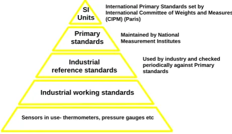
Traceability is the property of a result of a measurement or the value of a standard, whereby it can be related to stated ref-erences through an unbroken chain of comparisons all having stated uncertainties (see also Fig. A1).

NOTES

1. Traceability applies to the documentation process for all intermediate calibration steps, as well as to the check of all used intermediate calibration tools.

(9)

C. Waldmann et al.: Assessment of sensor performance 243

SI Units

Primary standards

Industrial reference standards

Industrial working standards

Sensors in use- thermometers, pressure gauges etc

International Primary Standards set by International Committee of Weights and Measures (CIPM) (Paris)

Maintained by National Measurement Institutes

Used by industry and checked periodically against Primary standards

Fig. A1. Standards are traceable through a chain of comparisons.

3. For measurements with more than one input quantity to the measurement function, each of the input quantities should itself be metrologically traceable.

A1.2 Measurement accuracy, accuracy of

measurement, accuracy

Accuracy describes the closeness of agreement between a measured value and the assumed true measurement result. The concept “measurement accuracy” is not associated with a numerical value. A measurement is said to be more accu-rate when it offers a smaller measurement error.

According to these definitions, traceable accuracy is not a standard term; it is not defined and, therefore, should be dis-carded. As a matter of fact, the term mixes two processes that have to be considered separately. GUM suggests spec-ifying the uncertainty as a numerical value to describe the “trueness” of the measurement.

A1.3 Measurement precision, precision

Precision specifies the closeness of agreement between in-dications or measured quantity values obtained by replicate measurements on the same or similar objects under specified conditions, which includes measurements taken under differ-ent conditions. This value is usually expressed numerically by terms of imprecision, such as standard deviation or vari-ance under specified measuring conditions. It should not be mistaken for measuring accuracy.

A1.4 Stability of a measuring instrument, stability

Stability is the property of a measuring instrument, whereby the continuously measured environmental conditions are kept constant in time. Stability may be quantified through a time interval where the measured value changed by a cer-tain amount or through quantifying a factor describing the temporal change.

This parameter is closely related to the conventional no-tion of accuracy. Although some manufacturers tend to spec-ify the residual deviations from the calibration function as

accuracy (in the conventional sense), it is obvious that the temporal stability also has to be taken into account. A nu-merical value for this can only be gained through repetitive calibrations.

A1.5 Resolution

Resolution describes the smallest change in a quantity being measured that causes a perceptible change in the correspond-ing indication. Resolution will depend on, for example, noise (internal or external).

A1.6 Sensitivity of a measuring system, sensitivity

Sensitivity is a relative measure describing the change in an indication of a measuring system and the corresponding change in a value of a quantity being measured. Sensitivity of a measuring system can depend on the value of the quan-tity being measured. The change considered in a value of a quantity being measured must be large compared with the resolution.

A2 Technology Readiness Levels summary according to

(Mankins, 2005)

A2.1 TRL 1 – basic principles observed and reported

This is the lowest “level” of technology maturation. At this level, scientific research begins to be translated into applied research and development. Examples might include stud-ies of basic propertstud-ies of materials (e.g., tensile strength as a function of temperature for a new fiber).

A2.2 TRL 2 – technology concept and/or application

formulated

Once basic physical principles are observed, then at the next level of maturation, practical applications of those character-istics can be “invented” or identified. For example, follow-ing the observation of high critical temperature (Htc) super-conductivity, potential applications of the new material for thin film devices (e.g., SIS mixers) and in instrument sys-tems (e.g., telescope sensors) can be defined. At this level, the application is still speculative; there is not experimental proof or detailed analysis to support the conjecture.

A2.3 TRL 3 – analytical and experimental critical func-tion and/or characteristic proof-of concept

(10)

A2.4 TRL 4 – component and/or breadboard validation

in laboratory environment

Following successful “proof-of-concept” work, basic tech-nological elements must be integrated to establish that the “pieces” will work together to achieve concept-enabling lev-els of performance for a component and/or breadboard. This validation must be devised to support the concept that was formulated earlier and should also be consistent with the re-quirements of potential system applications.

A2.5 TRL 5 – component and/or breadboard validation

in relevant environment

At this level, the fidelity of the component and/or bread-board being tested has to increase significantly. The basic technological elements must be integrated with reasonably realistic supporting elements, so that the total applications (component-level, sub-system level, or system-level) can be tested in a “simulated” or somewhat realistic environment.

A2.6 TRL 6 – system/subsystem model or prototype

demonstration in a relevant environment (pres-sure chamber, test basin, ocean)

A major step in the level of fidelity of the technology demon-stration follows the completion of TRL 5. At TRL 6, a rep-resentative model or prototype system or systems – which would go well beyond ad hoc, “patch-cord”, or discrete com-ponent level breadboarding – would be tested in a relevant environment. At this level, if the only “relevant environ-ment” is the ocean environment, then the model/prototype must be demonstrated in the ocean. Of course, the demon-stration should be successful to represent a true TRL 6. Not all technologies will undergo a TRL 6 demonstration; at this point, the maturation step is driven more by assuring man-agement confidence than by R&D requirements. The demon-stration might represent an actual system application, or it might only be similar to the planned application, but using the same technologies.

A2.7 TRL 7 – system prototype demonstration in a

space environment (in ocean sciences accordingly in an ocean environment)

TRL 7 is a significant step beyond TRL 6, requiring an actual system prototype demonstration in the ocean environment. In this case, the prototype should be near or at the scale of the planned operational system, and the demonstration must take place in the ocean. The driving purposes for achieving this level of maturity are to assure system engineering and devel-opment management confidence (more than for purposes of technology R&D). Therefore, the demonstration must be of a prototype of that application. Not all technologies in all systems will go to this level. TRL 7 would normally only be performed in cases where the technology and/or

subsys-tem application is mission critical and relatively high risk. Example from space science: the Mars Pathfinder Rover is a TRL 7 technology demonstration for future Mars micro-rovers based on that system design.

A2.8 TRL 8 – actual systems completed and “ocean

mission qualified” through test and demonstration

By definition, all technologies being applied in actual sys-tems go through TRL 8. In almost all cases, this level is the end of true “system development” for most technology ele-ments.

A2.9 TRL 9 – actual system proven through successful

mission operations

By definition, all technologies being applied in actual systems go through TRL 9. In almost all cases TRL9 marks the end of last “bug fixing” aspects of true “system development”.

Edited by: G. Griffiths

References

AMS Applied Microsystems: What is the difference

be-tween accuracy and precision?, online available at:

http://www.appliedmicrosystems.com/Products/Services/ ConductivityCalibration.aspx, 2008.

Bacon, S., Culkin, F., Higgs, N., and Ridout, P.: IAPSO standard seawater: definition of the uncertainty in the calibration pro-cedure and stability of recent batches, J. Atmos. Ocean. Tech., 24(10), 1785–1799, 2007.

Bates, N. R., Merlivat, L., Beaumont, L., and Pequignet, A. C.: Intercomparison of shipboard and moored CARIOCA buoy

sea-waterfCO measurements in the Sargasso Sea, Mar.Chem., 72,

239–255, 2000.

Denuault, G.: Electrochemical techniques and sensors for ocean research, Ocean Sci. Discuss., 6, 1857–1893, 2009,

http://www.ocean-sci-discuss.net/6/1857/2009/.

Dickson, A. G., Sabine, C. L., and Christian, J. R. (eds.): Guide

to best practices for ocean CO₂measurements, PICES Special

Publication 3, 191 pp., online available at: http://cdiac.ornl.gov/ oceans/Handbook2007.html, 2007.

Forchhammer, G.: On the composition of seawater in the different parts of the ocean, Philos. T. Roy. Soc. London, 155, 203–262, 1865.

Gouretski, V. and Koltermann, K. P.: How much is the

ocean really warming?, Geophys. Res. Lett., 34, L01610, doi:10.1029/2006GL027834, 2007.

GUM ISO: ISO/IEC GUIDE 98-3:2008, Guide to the expression of uncertainty in measurement, International Organisation for Stan-dardisation, Geneva, Switzerland, 2008.

Hamon, B. V.: The effect of pressure on the electrical conductivity of seawater, J. Mar. Res., 16, 83–89, 1958.

IFREMER: http://www.ifremer.fr/dtmsi/anglais/moyensessais/

(11)

ISO: ISO/IEC 17025:2005, General requirements for the compe-tence of testing and calibration laboratories, International Organ-isation for StandardOrgan-isation, Geneva, Switzerland, 2005. Janzen, C., Larson, N., Beed, R., and Anson, K.: Accuracy

and stability of Argo SBE 41 and SBE 41CP CTD conduc-tivity and temperature sensors, SEABIRD Technical paper, on-line available at: http://www.seabird.com/technical references/ paperindex.htm, 2008.

Kirkup, L. and Frenkel, B.: An Introduction to Uncertainty in Mea-surement, Cambridge University Press, 2006.

Kohlrausch, F.: Praktische Physik 1, 22nd edn., B. G. Teubner, Stuttgart, 1968.

Kr¨oger, S., Parker, E. R., Metcalfe, J. D., Greenwood, N., Forster, R. M., Sivyer, D. B., and Pearce, D. J.: Sensors for observing ecosystem status, Ocean Sci., 5, 523–535, 2009,

http://www.ocean-sci.net/5/523/2009/.

Mankins, J. C.: Technology Readiness Levels: A White Paper, Ad-vanced Concept Office, Office of Space Access and Technology, NASA, USA, 2005.

Millero, F. J., Feistel, R., Wright, D. G., and McDougall, T. J.: The composition of standard seawater and the definition of the reference-composition salinity scale, Deep-Sea Res. I, 55, 50– 72, 2008.

MMI project: http://marinemetadata.org, last access: 30 July 2009. NIST: NIST technical note 1297. Guidelines for evaluating and

ex-pressing the uncertainty of NIST measurement results, 1994. Pouliquen, S., Schmid, C., Wong, A., Guinehut, S., and

Bel-beoch, M.: Argo Data Management, Community White Paper, OceanObs’09 conference, Venice, September 2009.

Q2O project: http://q2o.whoi.edu/, last access: 30 July 2009.

QARTOD project: http://nautilus.baruch.sc.edu/twiki/bin/view, last access: 30 July 2009.

QUASIMEME project: http://www.quasimeme.org/nl/

25222726-Home.html, last access: 30 July 2009.

Riebesell, U., Fabry, V. J., and Gattuso, J.-P. (eds.): Guide

to Best Practices in Ocean Acidification Research and Data Reporting, European Project on Ocean Acidification, on-line available at: http://www.epoca-project.eu/index.php/Home/ Guide-to-OA-Research/, 2009.

Saunders, P., Mahrt, K., and Williams, R.: Standards and laboratory calibrations, in: WOCE Operations Manual, Part 3.1.3: WHP Operations and Methods, WOCE Hydrographic Programme Of-fice, Woods Hole Oceanographic Institution, Woods Hole, Mass., USA, July 1991.

Sullivan, D. B.: Time and frequency measurement at NIST: The first 100 years, Proc. 2001 IEEE Frequency Control Symposium, 4–17, June 2001.

UNESCO: Technical papers in marine science. The acquisition, cal-ibration and analysis of CTD data, No. 54, 1994.

VIM ISO: ISO/IEC GUIDE 99:2007(E/F), International vocabulary of metrology – basic and general concepts and associated terms (VIM), 2007.

WHOI: http://www.whoi.edu/page.do?pid=10360, last access: 30 July 2009.

Zielinski, O., Busch, J. A., Cembella, A. D., Daly, K. L., Engel-brektsson, J., Hannides, A. K., and Schmidt, H.: Detecting ma-rine hazardous substances and organisms: sensors for pollutants, toxins, and pathogens, Ocean Sci., 5, 329–349, 2009,