www.solid-earth.net/2/35/2011/ doi:10.5194/se-2-35-2011
© Author(s) 2011. CC Attribution 3.0 License.
Solid Earth
3-D thermo-mechanical laboratory modeling of plate-tectonics:
modeling scheme, technique and first experiments
D. Boutelier1,2and O. Oncken1
1Helmholtz Centre Potsdam, GFZ German Research Centre for Geosciences, Telegrafenberg, 14473 Potsdam, Germany 2School of Geosciences, Monash University, Victoria 3800, Australia
Received: 7 February 2011 – Published in Solid Earth Discuss.: 18 February 2011 Revised: 21 April 2011 – Accepted: 28 April 2011 – Published: 24 May 2011
Abstract. We present an experimental apparatus for 3-D thermo-mechanical analogue modeling of plate tectonic pro-cesses such as oceanic and continental subductions, arc-continent or arc-continental collisions. The model lithosphere, made of temperature-sensitive elasto-plastic analogue mate-rials with strain softening, is submitted to a constant temper-ature gradient causing a strength reduction with depth in each layer. The surface temperature is imposed using infrared emitters, which allows maintaining an unobstructed view of the model surface and the use of a high resolution optical strain monitoring technique (Particle Imaging Velocimetry). Subduction experiments illustrate how the stress conditions on the interplate zone can be estimated using a force sensor attached to the back of the upper plate and adjusted via the density and strength of the subducting lithosphere or the lu-brication of the plate boundary. The first experimental results reveal the potential of the experimental set-up to investigate the three-dimensional solid-mechanics interactions of litho-spheric plates in multiple natural situations.
1 Introduction
Plate tectonic processes are characterized by very large spa-tial and temporal scales. Consequently, geological data of-ten provide partial insights into their mechanics, and geo-dynamic modeling, using either experimental or numerical techniques, is routinely employed to better understand their development in space and time. The experimental model-ing technique is particularly efficient to investigate three-dimensional phenomena (Davy and Cobbold, 1991; Bellah-sen et al., 2003; Funiciello et al., 2003; Schellart et al., 2003; Cruden et al., 2006; Luth et al., 2010). However, in
multi-Correspondence to: D. Boutelier
ple experimental models, the rheological stratification of the lithosphere is simplified and the strength variations induced by the temperature gradient through the lithosphere are simu-lated using various analogue materials with different physical properties (Davy and Cobbold, 1991; Schellart et al., 2003; Cruden et al., 2006; Luth et al., 2010). A drawback of this simplification is that the mechanical properties are retained throughout the entire experiment regardless of temperature variations associated with vertical displacement.
Experimental modeling with temperature-sensitive ana-logue materials allows incorporating these temperature vari-ations and their mechanical consequences (Turner, 1973; Ja-coby, 1976; Jacoby and Schmeling, 1982; Kincaid and Ol-son, 1987; Chemenda et al., 2000; Rossetti et al., 2000, 2001, 2002; Wosnitza et al., 2001; Boutelier et al., 2002, 2003, 2004; Boutelier and Chemenda, 2008; Luj´an et al., 2010). A conductive temperature gradient imposed in the model litho-sphere controls the rheological stratification prior to mation (Boutelier et al., 2002, 2003, 2004). During defor-mation, heat is naturally advected and diffused so that tem-perature and strength change with time in various parts of the model lithosphere (e.g. in the subducted lithosphere). How-ever, due to the complexity of the thermo-mechanical ana-logue modeling technique, most thermo-mechanical models used a two-dimensional approximation.
infrared emitters
PIV camera stepper motor
thermal probes
force sensor
electric heater PIV camera
upper plate
lower plate
asthenosphere
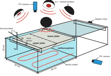
Fig. 1. 3-D sketch of the experimental set-up. Two lithospheric plates made of hydrocarbon compositional systems rest on the asthenosphere
modeled by water. A temperature gradient is imposed in the model lithosphere. A thermo-regulator receives the temperature of the water and at the model surface measured by 2 thermal probes and automatically adjusts the length of the heat pulses produced by the lower electric heater and 4 infrared emitters. Plate convergence is imposed at a constant rate and a force sensor installed in the back of the upper plate measures the force in the horizontal convergence parallel direction. Model strain is monitored using a Particle Imaging Velocimetry system imaging the model surface. A second optional camera is employed to follow the model evolution from the side.
the surface of the model lithosphere is controlled and main-tained using infrared emitters, which permit an unobstructed view of the model surface (Fig. 1). In turns, this allows us-ing the Particle Imagus-ing Velocimetry (PIV) technique to pre-cisely monitor, from above, the model deformation in time and space (Hampel, 2004; Adam et al., 2005; Hoth et al., 2006, 2007, 2008).
2 General modeling scheme
The lithosphere is the superficial shell of the Earth capable of undergoing large quasi-rigid horizontal displacements with strain-rates far lower than those experienced by the under-lying asthenosphere (Anderson, 1995). This definition pro-vides the general framework for our modeling. Since the vis-cosity of the asthenosphere is several orders of magnitude lower than the effective viscosity of the lithosphere (Mitro-vica and Forte, 2004; James et al., 2009), it can only exert a small shear traction on the base of the lithosphere (Bokel-mann and Silver, 2002; Bird et al., 2008). Hence, when studying deformation in a limited area around the subduc-tion zone we can neglect the local effect of viscous coupling between the lithosphere and asthenosphere and replace its larger-scale effect by the action of a piston. Consequently
the asthenosphere can be modeled with a low-viscosity fluid (water), whose unique role is to provide hydrostatic equilib-rium below the lithosphere. We acknowledge that the role of the asthenosphere is currently simplified (Bonnardot et al., 2008a). The viscous interaction between the lithosphere and asthenosphere will be implemented in a later developmen-tal stage of our experimendevelopmen-tal set-up. However, before im-plementing viscous interactions, it is necessary to develop a three-dimensional apparatus standing on the earlier two-dimensional thermo-modeling apparatus.
oceanic lithosphere with a 3-layer model in which the upper-most layer is elasto-plastic with high brittleness, the second layer is more ductile and the bottom layer is elasto-visco-plastic. In this study, the oceanic lithosphere is simplified and represented by one unique elasto-plastic ductile layer whose strength, however, decreases with depth because of the imposed temperature distribution. The latter is simpli-fied because we impose a linear conductive gradient through the lithosphere (i.e. no heat production), and an isothermal sub-lithospheric mantle (i.e. vigorous convection).
Finally, since we are interested in the large deformation of the lithosphere, we must also consider the material strain-softening behavior required in order to produce and main-tain lithospheric-scale shear zones. In the brittle layers of the lithosphere, localization is a natural consequence of the deformation mechanism. However, strain localization in the ductile regime is not fully understood. It may be promoted by strain softening mechanisms such as dynamic recrystal-lization and shear heating (Poirier, 1980; White et al., 1980; Rutter and Brodie, 1988; Mont´esi and Zuber, 2002; Hartz and Podladchikov, 2008), but the softening functions associated with these mechanisms are still being debated. An equivalent efficient strain localization process (up to∼50 % softening) is obtained in our model lithosphere using specially designed strain-softening elasto-plastic materials.
3 Scaling requirements
The principle of analogue modeling is based on scaling laws, in which geometric, kinematic and dynamic similarity be-tween the natural prototype and the model are achieved by scaling-down lengths, time and forces (Buckingham, 1914; Ramberg, 1967; Davy and Cobbold, 1991; Shemenda, 1994). When scaling relationships are fulfilled, the model behaves mechanically like the prototype but is manageable in a lab-oratory, and the effects of various key parameters can then be tested using multiple, carefully designed, built and moni-tored experiments.
For conveniency the model lithosphere must be relatively small. Hence, we decided that 1 cm in the model represents 35 km in nature, which yields a length scaling factorL∗= Lm/Ln=2.86×10−7.
The scaling of the all densities in the model is already set by our choice of using water to represent the astheno-sphere. The scaling factor for densities is ρ∗=ρm/ρn= 3.08×10⁻¹as 1000 kg m−3 represents 3250 kg m−3. Con-sequently, an old, dense, oceanic lithosphere can be modeled using a material with a density of 1040 kg m−3 represent-ing 3380 kg m−3in nature (i.e. with a negative buoyancy of 130 kg m−3), while the low-density continental crust can be modeled with material having a density of 860 kg m−3 repre-senting 2795 kg m−3in nature.
The scaling of stress is already set by the scaling of hy-drostatic pressure ρ g z where depth z scales with length. Since the experiments are produced with normal gravi-tational acceleration (i.e. g∗=1 or gm=gn= 9.81 m s−2), σ∗=σm/σn=ρ∗×L∗=8.79×10−8 and a flow stress of
∼10 MPa at the bottom of the lithosphere must be∼1 Pa in the model, while a flow stress of 500 to 1000 MPa in the stronger part of the lithosphere must be 44 to 88 Pa in the model. Therefore, the analogue material employed to model the oceanic lithosphere should have a strength∼1 to
∼100 Pa from the bottom to the top.
Before plastic failure, the lithosphere deforms elastically with a shear modulusGnof∼1 to 10×1010Pa (Dziewon-ski and Anderson, 1981). Since the dimension ofGis that of a stress, it must be scaled by the same ratio: σ∗. There-fore, the model shear modulus should be of the order of∼1 to 10×103Pa. However, measuring the shear modulus of a very weak material proved to be challenging and therefore the shear modulus could only be measured for low tempera-tures corresponding to the surface of the model lithosphere. Hence, we must acknowledge that the elastic properties are only approximately scaled.
The scaling of time is chosen in order to scale the temper-ature variations associated with deformation. The imposed velocity controls the advection of heat in the model, which must be balanced with the diffusion. In order to maintain the same balance between advection and diffusion as in nature, the dimensionless ratio VL/κ, withV being the velocity, L the length, andκ the thermal diffusivity, must be the same in the model and nature (Chemenda et al., 2000). Since the scaling of length has been set already, the thermal diffusiv-ity of the analogue materials controls the scaling of velocdiffusiv-ity and therefore of time. The later is simply defined in a kine-matic sense using the dimensionless ratio Vt/Lwheretis the time. The scaling of velocity and time is further detailed in Sect. 4.5.
4 Analogue materials
Table 1. Parameter values adopted for the models (arefers to Exp. 2 andbrefers to Exp. 3), scaled to nature and scaling factors. The plastic strength of the materials decreases with depth in each layer. In this table we indicate the strengths averaged over the layer thickness.
Parameters Model Nature Scaling factor
ThicknessH (m) 2–3b×10−2±2×10⁻⁴ 7–10.5b×104 2.86×10⁻⁷ Plastic strengthσ(Pa) 25–40b±2 25–40b×108 8.79×10⁻⁸ Elastic shear modulusG(Pa) ∼1×10¹⁰ ∼1×10³ 8.79×10⁻⁸ Lithosphere densityρl(kg m−3) 1.0–1.04a,b×103±4.8×100 3.25–3.38a,b×103 3.08×10⁻¹ Asthenosphere densityρa(kg m−3) 1.0×10³±2×100 3.25×10³ 3.08×10⁻¹ Thermal diffusivityκ(m2s−1) 2.8×10⁻⁸±1.0×10⁻⁹ 1.0×10⁻⁶ 2.8×10⁻² VelocityV (m s−1) 2.50×10⁻⁴±2.0×10⁻⁶ 2.54×10⁻⁹ 9.8×10⁴ Timet(s) 3.15×10¹³ 9.2×101 2.92×10⁻¹²
4.1 Composition
The materials are composed of various quantities of paraf-fin and microcrystalline waxes, Vaseline, and parafparaf-fin oil held together with a highly branched alphaolefin polymer. The density is adjusted with the addition of a clay pow-der, which binds with the oil-based matrix via a water-in-oil surfactant (phosphatidylcholine). The material employed for the neutrally-buoyant mantle lithosphere of Experiment 1 has the following proportions: Vaseline (32.2 wt %), min-eral oil (32.2 wt %), clay powder (23 wt %), paraffin wax (6.3 wt %), alpha-olefin polymer (4.5 wt %), microcrystalline paraffin wax (1.5 wt %) and phosphatidylcholine (0.3 wt %). 4.2 Mechanical testing
The mechanical properties of the materials have been mea-sured at the Helmholtz-Zentrum Potsdam (GFZ) using a Rheotec RC20 CPS rheometer with cone-and-plate geome-try. The materials are liquid at a temperature greater than or equal to the melting point (45–50◦C). To measure the me-chanical properties of the materials at temperatures within the range 37–43◦C used in the experiments, the sample is first melted on the heating bottom plate of the rheometer and the rheometer head is slowly lowered into the sample. The temperature is then slowly lowered to 20◦C and the sample is kept at ambient temperature until full strength is developed. The temperature is finally slowly increased to and maintained at the desired temperature of measurement. This protocol al-lows having full coupling between the sample and both the bottom plate and rheometer head.
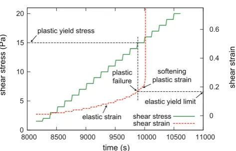
The material mechanical behavior at a specific tempera-ture is characterized in simple shear using a series of succes-sive creep tests. A constant shear stress is imposed on the sample for 120 s and then it is ramped up. With low shear stresses, the materials behave elastically and shear strain in-creases with shear stress (Fig. 2). When the yield stress is reached, shear strain rapidly increases while the shear stress
0 5 10 15 20
8000 8500 9000 9500 10000 10500 11000
0 0.2 0.4 0.6
sh
e
a
r
st
re
ss
(Pa
)
sh
e
a
r
st
ra
in
time (s)
shear stress shear strain plastic
failure
elastic strain
softening plastic strain
elastic yield limit plastic yield stress
Fig. 2. Procedure employed to measure the material’s mechanical
properties. A constant shear stress is imposed on the sample during each time step, and then ramped up. For low shear stresses, the shear strain increases synchronously with the shear stress increase and then remains stable. When the plastic yield stress has been reached, the shear strain increases rapidly during the constant-stress creep step.
is maintained constant (Fig. 2). This type of test allows char-acterizing the elastic shear modulus quantitatively, the plas-tic yield stress, and the softening/hardening behavior quali-tatively .
4.3 Elastic properties
0 0.005 0.01 0.015 0.02 0.025 0.03
20 30 40 50 60 70 80 90 100
cumulative elastic strain
shear stress (Pa) experimental data (T=37C)
linear fit J= 1/G x W
with G= 2866 Pa
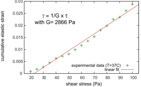
Fig. 3. Strain-stress curve obtained using the shear strain
augmenta-tion synchronous with the shear stress growth prior to reaching the plastic yield stress.
elastic properties but if the shear stress is increased in too large steps, the precision on the yield stress is not satisfac-tory. Finally, another restriction on the measurement of the elastic properties arises when the plastic yield stress is small. Then only a few data points can be collected, which is in-sufficient to derive a meaningful linear regression and thus elastic shear modulus. Consequently, we adopted the follow-ing strategy:
– For high temperatures (≥39◦C), when the material is weak, the mechanical test is performed using small shear stress steps (1 or 2 Pa) and the elastic properties are not derived.
– For low temperatures (≤39◦C) the tests are conducted with larger shear stress steps allowing measurement of the elastic properties.
The results reveal that the shear modulus decreases with tem-perature increase but remains in the range of 1000 to 3000 Pa, which scales to 1.14 to 3.4×10¹⁰Pa in nature (Fig. 3). Char-acterisation of the elastic properties thus remains incomplete; however, the presented values of the shear modulus are ro-bust since oscillatory tests (see Boutelier et al., 2008, for pre-cisions on oscillatory tests) also showed a dynamic storage modulusG0(equivalent toGin dynamic tests) with the same magnitude (∼1500 Pa).
4.4 Plastic yield stress
The plastic yield stress is measured using the same series of successive creep tests used to characterize the elastic shear modulus. When the imposed shear stress reaches or over-comes the plastic yield stress, deformation beover-comes rapidly much larger and it continues during the entire creep step, al-lowing the rheometer to measure a shear rate.
We qualitatively characterized the softening/hardening be-havior using the creep test, during which failure occurred. In this creep test, the shear stress is constant and is equal to the yield stress. We observed that the shear strain in-crease upon failure is best fitted with a degree-3 polynomial function (i.e. constant acceleration) which is characteristic of plastic softening (Shemenda, 1992). This allows us to af-firm that our materials are softening and comparable to the materials developed by A. Chemenda employed in earlier 2-D thermo-mechanical experiments (Chemenda et al., 2000; Boutelier et al., 2002, 2003, 2004; Boutelier and Chemenda, 2008). These materials have been shown to soften by 20 to 50 % depending on temperature (Shemenda, 1992, 1993, 1994; Boutelier, 2004).
The rheological stratification of the model lithosphere prior to deformation is obtained when the strength of all the materials constituting the various layers of the lithosphere is known for all the temperatures imposed inside the model lithosphere. In the presented experiments, the lithosphere is made of one single mantle layer and therefore the strength of one single material must be known. Figure 4 shows the vari-ations of the plastic yield stress of our material for the tem-peratures 38 to 43◦C. However, in the presented experiments the surface temperature was 39◦C and the temperature of the asthenosphere was 42◦C. Within this temperature range, the strength decreases from 50 to 6 Pa (see inset in Fig. 4), which corresponds to a decrease from 5.7×10⁸to 6.8×10⁷Pa in nature.
Our materials exhibit ductile plastic failure, as permanent deformation can be observed prior to failure in the stress-time diagram and ductile flow can be observed around the fault zone. However, the amount of plastic deformation prior to failure decreases with the temperature. Therefore, our ma-terials become more brittle (i.e. deformation is more local-ized) with lower temperature. Brittle plastic failure should prevail near the model surface. However, it is not presently possible to implement brittle behavior in our experiments be-cause brittleness is only obtained for very low temperatures, when the materials are too strong. Furthermore, even if we were able to modify our materials in order obtain more brit-tle behavior near the surface together with a low strength, we would not be able to reproduce the strength increase with depth in this part of the model as our materials are sensitive to temperature but not pressure. We acknowledge that the strength envelope is approximated near the model surface, and that deformation of the near surface is best modeled with granular materials (e.g. Corti, 2008; Malavieille and Trul-lenque, 2009; Malavieille, 2010).
4.5 Thermal diffusivity
0 20 40 60 80 100 120 140
38 39 40 41 42 43
yi
e
ld
st
re
n
g
th
(Pa
)
temperature (˚C) 2.0 1.0 0.5
1.5
39 42 0 10 20 30 40 50 temperature (°C) yield strength (Pa)
d
e
p
th
(cm)
lithosphere
asthenosphere
Fig. 4. Evolution of the plastic yield stress with temperature. The
plastic yield stress decreases with increasing temperature. Inset: Once the temperature gradient in the model lithosphere is known, the experimental curve is used to draw the strength envelop of the model lithosphere prior to deformation.
high temperature above the melting point and allowed to cool down. The heat loss is restricted to the upper surface only and the temperature is monitored at a known depth below the centre of the upper surface. In these conditions, a 1-D half-space cooling approximation is reasonable and the data can be fitted with the analytical solution (Turcotte and Schubert, 1982):
T (z,t )=Te+(Ti−Te)×erf
z
2√κt
(1) whereT (z,t )is the temperature at depthzand timet,Teis the external temperature,Tiis the initial temperature and κ is the thermal diffusivity. For our compounds, the best fit is obtained with a thermal diffusivity of 2.8×10⁻⁸m2s−1 (Fig. 5). Assuming that the modeled rocks have a thermal diffusivity of 1×10⁻⁶m2s−1(Turcotte and Schubert, 1982), thenκ∗=2.8×10⁻²and a scaling factor for velocityV∗= Vm/Vn=κ∗/L∗=9.8×104can be derived from the dimen-sionless ratio VL/κ. This scaling factor means that a natu-ral subduction velocity of 8 cm yr−1(i.e. 2.54×10⁻⁹m s−1) is 0.25 mm s−1in the model. The scaling factor for time is thereforet∗=tm/tn=L∗/V∗=2.92×10−12, which implies that 1 Ma in nature (i.e. 3.15×10¹³s) is 92 s in the model.
5 Experimental apparatus
The experimental set-up comprises a polycarbonate tank 50×50×30 cm3filled with water representing the astheno-sphere (Fig. 1). The model lithospheric plates are built in a mold 40×40×6 cm3. The experimental tank is sufficiently larger than the model plates (5 cm on each side) that the sides can be considered to be free. The experimental set-up in-cludes two new features that are presented here. The surface
43 44 45 46 47 48 49
0 1000 2000 3000 4000 5000 6000 7000
te
mp
e
ra
tu
re
(˚C
)
time (s)
experimental data 1D cooling solution
Fig. 5. The material thermal diffusivity is fitted with a 1-D
cool-ing solution. The best fit provides a thermal diffusivity of 2.8×
10−8m2s−1.
temperature is maintained without obstructing the view of the model surface for optical strain monitoring and the horizon-tal convergence parallel force is measured at the back of the upper plate.
5.1 Particle imaging velocimetry and surface heating A major difficulty with 3-D experimental models is monitor-ing the model deformation in its center. Because we wish to explore three-dimensional processes, the model is likely to include along-strike variations of the initial conditions which make the deformation process different in the center and along the sides. Therefore the model side views are not sufficient and it is necessary to monitor strain from the top. Precise spatio-temporal strain monitoring is obtained using the Particle imaging velocimetry (PIV) technique (Hampel, 2004; Adam et al., 2005), a non-intrusive method for ac-curate measurement of instantaneous velocity/displacement fields using an image correlation technique. Our PIV system is equipped with 10 megapixel cameras enabling a spatial resolution of the displacement below 0.1 mm while the tem-poral resolution is 0.1 s. However, in the presented experi-ments the successive PIV images are taken at a time interval of 2 to 5 s, which is sufficient to monitor the slow model de-formation (<0.25 mm s−1).
52 50 48 46 44 42 40 38 36 34 32 30 28 26 24 22
10 cm
conductive gradient through the lithosphere
3
4 36 40 42
34 36 38 40
T(oC) T (oC)
T (oC)
model lithosphere
m
o
d
e
l
a
s
th
e
n
o
s
p
h
e
re
Fig. 6. Infrared image of the model surface. The homogeneity of
the surface temperatureTsis measured using an infrared camera. After 3 h of heating, the temperature field shows only one small ridge associated with the plate boundary. The temperature varia-tions across the model surface are otherwise smaller than 0.2◦C. In this test the surface temperature was 38◦C and the temperature of the asthenosphere was 42◦C. In the bottom right darker corner, the model is masked.
with thermo-mechanical models was to impose the surface temperature Ts while maintaining an unobstructed view of the model surface. We solved this problem using infrared emitters coupled to a thermal probe and a thermo-regulator (Fig. 1). Four 250 V/250 W infrared emitters equipped with large diffusers were placed 60 cm above the 4 corners of the experimental tank and are oriented towards the center of the model surface. The infrared emitters do not produce any vis-ible light and the PIV cameras do not see the emitted infrared waves. Therefore, the heating system is perfectly invisible to the PIV strain monitoring system. The surface temperature is continuously measured by a thermal probe in one location and the temperature value is given to the thermo-regulator which, depending on the temperature difference between the set temperature and measured temperature, adjusts the length of the pulses emitted by the infrared bulbs. This set-up al-lows having a surface temperature field that is relatively con-stant (±0.1◦C) in time and homogeneous (±0.2◦C) in space (Fig. 6). A similar system controls the temperature of the model asthenosphere, however the heating element is a sim-ple 250 V/2000 W electric resistance placed at the bottom of the tank, as in previous thermo-mechanical experimental set-ups (Chemenda et al., 2000; Boutelier et al., 2002, 2003, 2004; Boutelier and Chemenda, 2008).
5.2 Force monitoring
In order to better understand the stress regime in the arc area during the processes of subduction and/or arc-continent collision, we placed a force sensor in the back of the
up-per plate. The upup-per plate rests against a vertical plate at-tached to the back-wall of the experimental tank via a 2.5 N force sensor. This set-up allows measuring the force in the horizontal convergence-parallel direction. In this study we present a quantitative analysis of the effects of slab buoy-ancy, flexural rigidity and interplate friction on the interplate stresses and produced stress/strain regimes in the arc area during oceanic subduction. However, the measurement of the horizontal convergence-parallel stress is only really use-ful in a quantitative manner when the model is cylindrical and the same process occurs at the same time across the entire width of the model. It is therefore best used in preliminary experiments such as presented in this study. The rationale for placing this force measurement system is that the effects of some parameter values (densities, temperatures) on the in-terplate stresses can be measured in cylindrical experiments and then the same effects can be assumed in more complex non-cylindrical models.
Our modeling apparatus is computer-controlled and a sin-gle computer simultaneously reads the force measured at the back of the upper plate and imposes the rate of the piston. The force sensor is interrogated 30 times per second and the computer can either store the values and maintain conver-gence rate at a set value or it can adjust the converconver-gence rate in order to achieve a set force. We have not yet fully tested this system and there are parameters that remain to be investi-gated/tuned. For example, we presently don’t know the max-imum acceleration that should be allowed or how we should filter the force signal in real time in order to ignore the high-frequency force variations that do not pertain to the model mechanics. We will further discuss the future development of the modeling apparatus and in particular of dynamic mod-els in the discussion section.
6 Results
6.1 Simple oceanic subduction experiments
as the density and flexural rigidity of the lower plate or the interplate friction. Here we present two simple experiments in which we varied the density of the subducting slab and the interplate friction.
In Experiment 1, the subducting lithophere is neutrally buoyant (ρl=ρa) and the plate boundary is lubricated with a 0.1 mm-thick layer of parafine oil (η=0.5 Pa s). We as-sume that in this situation the shear traction is null. Figure 7 shows the model surface photographs at various stages with the velocity vectors derived from the image correlation tech-nique and the incremental (i.e. between 2 successive images) convergence-parallel normal strain (Exx). The PIV monitor-ing yields vectors that are very honogeneous in both direc-tion and magnitude within the subducting plate (Fig. 7a–c). The model plate therefore moves as a quasi-rigid body. The upper plate does not move and is only slightly deformed dur-ing subduction initiation (Fig. 7a). Therefore plate conver-gence is only accomodated by sliding along the interplate zone. In the conditions of this experiment, the normal stress measured at the back of the upper plate is the horizontal com-pression due to the flexural rigidity of the plate (Shemenda, 1993). During subduction initiation, the stressσxxincreases to a value of∼12 Pa and then remains approximately at this level during the rest of the experiment (Fig. 8). This normal stress is due to the non-hydrostatic normal stressσn exerted
on the plate boundary by the subducting plate because it re-sists bending. Knowing the value of the normal stressσxx within the upper plate we can estimate the horizontal com-ponent(Fp)hof the pressure forceFp. Since we also know the inclinationα, widthWand thicknessH of the plate, we can estimate the magnitude of the pressure forceFpand the depth-averaged non-hydrostatic normal stressσ¯nfrom which
it derives (Fig. 10a):
(Fp)h=σxx×H×W=9.3×10⁻²N (2) then
Fp=(Fp)h/cos(α)=1.08×10−1N (3) and
¯ σn=
Fp×cos(α)
H×W =12 Pa (4)
Note that it is possible to increase or decrease the flexural rigidity of the subducting plate and thus the depth-averaged non-hydrostatic normal stress by adjusting, for example, the temperatures (and thus strength) in the model.
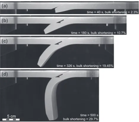
In Experiment 2, the subducting lithosphere is denser than the asthensphere by 4 %. Consequently, the slab exerts a pull on the plate boundary which subtracts from the com-pression due the flexural rigidity. Also, since the viscosity of our model asthenosphere is very low and the trailing edge of the plate is fixed, the negative buoyancy of the subduct-ing lithosphere leads to the formation of a very steep slab (Fig. 9). In this experiment, we also increased the interplate
friction by sifting a small amount of sand grains at the sur-face of the subducting plate. Therefore, the normal stressσxx recorded at the back of the upper plate reflects the sum of the compression due the flexural rigidity, the tension due to the slab pull and the compression due to the increased fric-tion. Of these 3 key parameters, only one is known from Ex-periment 1. However, the effects of the slab negative buoy-ancy and high interplate friction evolve differently in time. At the begining of the experiment, the effect of the slab pull force is minor because the slab is not developped yet. Con-sequently we recorded a normal stressσxxthat is larger than that recorded in Experiment 1 (Fig. 8). Assuming that the ef-fect of the slab pull force can be neglected at the begining of the experiment, the stress difference between experiments 1 and 2 must be due to increased friction. We can therefore estimate the horizontal component of the friction forceFf (Fig. 10c):
(Ff)h=σxx×H×W−(Fp)h (5) then
Ff=(Ff)h/sin(α)=1.16×10−1N (6) and finally the depth-averaged shear stress
¯
τ=Ff×cos(α)
W×H =13 Pa (7)
After a short plateau, the recorded normal stressσxx de-creases and it keeps decreasing until the end of the experi-ment. The steep geometry of the subducted slab (Fig. 9) re-veals that the decrease of the horizontal compression is due to the slab pull force exerted by the subducting slab on the interplate zone. In the presented experiment the horizontal stress becomes very close to zero near the end of the exper-iment. In other similar experiments it has been possible to obtain a tension. However, the magnitude of the tension can-not be very large because the plates are can-not strongly attached to the piston and back wall and would, under the effect of a large tension, detach and move towards the center of the experimental tank. σxx is due to the combined effects of the horizontal component of the pressure force due to the slab negative buoyancy (Fp2), the horizontal components of the pressure force due to flexural rigidity (Fp1) and the friction force (Ff):
σxx×H×W =(Fp1)h+(Ff)h−(Fp2)h (8) We estimate the pressure force due to the slab negative buoy-ancyFp2(Fig. 10b):
Fp2 = (Fp2)h/cos(α) = −2.24×10⁻¹N (9) and the associated depth-averaged non-hydrostatic normal stressσ¯n
¯ σn=
Fp2×cos(α)
0.25 mm/s
(a) (b) (c)
-0.15 -0.14 -0.13 -0.12 -0.11 -0.1 -0.09 -0.08 -0.07 -0.06 -0.05 -0.04 -0.03 -0.02 -0.01 0
Exx
upper plate lower plate
plate boundary x
y
5 cm
time = 186 s, bulk shortening = 10% time = 326 s, bulk shortening = 18% time = 608 s, bulk shortening = 34%
Fig. 7. Surface views of the model in Experiment 1. Correlation of successive images allows the derivation of a velocity field (arrows). Note
that for clarity only 1/4×1/8 of all the velocity vectors are presented here. From the velocity field the normal strain in the convergence directionExxis derived. The magnitude ofExxis calculated using the displacement field computed between 2 successive images taken 5 s apart (i.e. divide by 5 to obtain time-averaged strain rate). Both the vector field and the strain field reveal that the both plates are largely undeformed and convergence is accommodated by sliding of the lower plate under the upper plate.
-5 0 5 10 15 20 25 30 35
0 100 200 300 400 500 600 700 800 900
σ
(Pa
)
time (s)
Experiment 1 Experiment 2
Fig. 8. Convergence parallel normal stress recorded in the back of
the overriding plate in Experiments 1 and 2. In Experiment 1, the recorded compressive stress is due to the flexural rigidity of the plate which resists bending. In Experiment 2, the stress at the beginning of the experiment is due to the combined effects the flexural rigidity and high interplate friction. However, during Experiment 2, the compressive stress decreases because the subducted slab becomes longer and its pull becomes stronger.
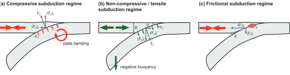
The presented data clearly show that (1) the experimen-tal apparatus allows modeling plates which move with lit-tle/no internal deformation, (2) the monitoring technique al-lows precise spatial resolution of model deformation, and (3) the measured stress allows defining 3 end-member sub-duction regimes characterised respectively by compression due to the bending strength of the subducting plate, tension due to the negative buoyancy of this plate and compression due to the interplate friction (Fig. 10).
(a)
(b)
(c)
5 cm
(d)
time = 40 s, bulk shortening = 2.3%
time = 180 s, bulk shortening = 10.7%
time = 326 s, bulk shortening = 19.45%
time = 500 s bulk shortening = 29.7%
Fig. 9. Side images of the model in Experiment 2. The negative
buoyancy of the subducted lithosphere tends to steepen the slab.
6.2 Forced subduction initiation experiment
plate bending
negative buoyancy
(a) Compressive subduction regime (b) Non-compressive / tensile
subduction regime
(c) Frictional subduction regime
Fp (Fp)v
(Fp)h
Fp (Fp)v
(Fp)h
Ff (Ff)v (Ff)h
τ σn
σn
α Η
Fig. 10. Sketches of the main subduction regimes and the key parameters causing them. A compressive subduction regime is caused by the
flexural rigidity of the lower plate which resists bending (a). However, this regime is only obtained when the slab is neutrally buoyant because the negative buoyancy of the subducted lithosphere exerts a tensile non-hydrostatic normal stress on the plate boundary which generates a horizontal tension in the upper plate (b). Finally, a horizontal compression can also be generated because of a large interplate friction (c).
thermal gradient is higher, which makes the model litho-sphere at shallow depth above the notch weaker than else-where in the model. The model plate is shortened at the same constant rate as in Experiments 1 and 2, which results in de-formation of the plate near the notch and finally the forma-tion of a subducforma-tion zone (Fig. 11). We do not pretend that the presented mechanism is at play in nature during subduc-tion initiasubduc-tion. This experiment is realized in order to ob-serve how strain localization due to plastic strain-softening can lead to the formation of a lithospheric-scale shear zone in our model lithosphere. Furthermore, we use this experi-ment to illustrate how the PIV system allows having a pre-cise monitoring of when the various deformation structures are active.
The experiment being cylindrical is also monitored from the side. Successive side views revealed that shortening is accommodated by two conjugate shear zones nucleated from the roof of the notch and resulting in the formation of a pop-up above it (Fig. 11a). With further shortening, the shear zone located left of the notch becomes dominant, accommo-dates most of the shortening and thus forms a new subduction zone (Fig. 11b–f). However, the side views also reveal that both plates underwent some shortening near both the piston and the back wall (Fig. 11b).
The PIV monitoring of the model surface allows us to de-scribe more precisely the evolution of model deformation in space and time. The shortening indeed started with the formation of two oppositely dipping shear zones around the notch (Fig. 12a). However, before the shear zone on the left side of the notch became dominant, another shear zone is also created near the back wall (Fig. 12a). At this point, none of the shear zones appear to run entirely across the width of the model plate. This shortening is accommodated by the net-work of shear zones and distributed across the entire model. PIV monitoring reveals that this process of strain accommo-dation does not perpetuate. The shear zone located to the right of the notch becomes inactive while the shear zones
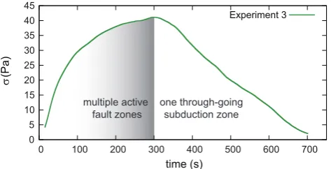
located left of the notch and near the back wall propagate laterally (Fig. 12b). It is the advantage of using the PIV tech-nique to be able tell when, during the experiment, a structure becomes inactive and when another one becomes active or more important. The shortening is accommodated by fewer and fewer structures as strain weakens the material. Finally the shear zone located near the back wall also becomes in-active (Fig. 12c) and shortening is solely accommodated by one shear zone which evolves into a new subduction zone (Fig. 12c–d). The strain localization process is accompanied by a diminution of the stress recorded at the back of the upper plate once the main fault zone runs across the entire model width and has recorded sufficient strain to be significantly weakened (Fig. 13). The recorded diminution is also due to the fact that, since the mantle lithosphere material is slightly denser than the asthenosphere, the formation of a slab leads to a slab pull force whose action diminishes the horizontal compression.
7 Discussion
7.1 A framework for modeling lithospheric plate interactions in a convergent setting
time = 120 s bulk shortening = 7%
time = 0 s bulk shortening = 0%
time = 300 s bulk shortening = 19%
time = 415 s bulk shortening = 26%
time = 536 s bulk shortening = 34%
time = 680 s bulk shortening = 42%
5 cm (a)
(b)
(c)
(d)
(e)
(f)
Fig. 11. Side views of Experiment 3. The model is composed of one
single layer of mantle lithosphere with a notch in the middle of the plate’s length. The side pushed by the piston (i.e. right-hand side) becomes the upper plate while the other side slides down a newly created subduction zone.
modeling of the lithospheric plates interaction is required. Furthermore, since the targeted geodynamic problems are likely to include large vertical movements of the crust and/or lithosphere and hence significant temperature variations, it is important that the modeling framework includes the spatial and temporal strength variations associated with temperature changes.
The presented experiments are large but cylindrical mod-els since we did not implement any lateral (i.e. along-strike) variations of the model structure, mechanical properties or any other initial or boundary conditions. We presented cyldrical models because such simpler models allow us to in-troduce the key parameters controlling the solid-mechanics interaction of the lithospheric plates during the process of oceanic subduction. Furthermore, these experiments per-mit detailing the advantages and liper-mitations of our approx-imations and modeling set-up. However, the new apparatus clearly has the potential for modeling the above-mentioned non-cylindrical geodynamic problems. The present study should therefore be seen as a first step in a series designed to study such three-dimensional non-cylindrical processes, rather than the final step.
7.2 Quantitative stress and strain monitoring
One key advantage of the employed experimental setup is the ability to precisely monitor the model deformation from above using the 2-D PIV technique. Because we aim at pro-ducing complex 3-D models, we cannot rely on side obser-vations of the model as in previous 2-D thermo-mechanical experiments (Boutelier et al., 2002, 2003, 2004). The high spatial and temporal resolution of the PIV technique allows a more precise monitoring of the model deformation than conventional strain marker analysis (Boutelier and Cruden, 2008). Theoretically, it is also possible to monitor the verti-cal displacement of the model surface using 2 cameras pro-viding a stereoscopic view of the model surface (Adam et al., 2005; Riller et al., 2010). This new advance in monitoring technology would be very advantageous because the verti-cal motion of the model surface can be linked to the dis-tribution of stresses along the plate boundary (Shemenda, 1992), compared with numerical modeling results (Hassani et al., 1997; Bonnardot et al., 2008a,b) or compared with nat-ural data such as long-term uplift/subsidence derived from sedimentary record (Matsu’ura et al., 2008, 2009; Stefer et al., 2009; Hartley and Evenstar, 2010), short-term up-lift/subsidence derived from GPS/Coral reefs dating (Tay-lor et al., 2005; Matsu’ura et al., 2008, 2009) or gravity anomalies (Shemenda, 1992; Song and Simons, 2003). How-ever, the produced topography is very small (∼1–2 mm) and the distribution of passive markers is not sufficiently large to permit reliable stereoscopic imaging and therefore verti-cal motions. A possible workaround would be to employ a three-dimensional video laser to scan the model surface at regular time intervals during the experiment and convert the data to digital elevation models (Willingshofer et al., 2005; Willingshofer and Sokoutis, 2009; Cruden et al., 2006; Pysklywec and Cruden, 2004; Luth et al., 2010). The strain monitoring system in its present development allows pre-cise spatio-temporal resolution of the 2-D deformation of the model surface. This allows tracking when, during the experiment, the various deformation structures are active. Coupled with stress monitoring and the ability to produce vertical sections through the frozen model in the end of the experiment (Boutelier et al., 2002, 2004; Boutelier and Chemenda, 2008), the strain monitoring system provides the required data to understand how stress and strain develop in the model.
7.3 Imposing a subduction regime in non-cylindrical thermo-mechanical experiments
5 cm
0.25 mm/s
(d) (c)
(b) (a)
x
y -0.04
-0.035 -0.03 -0.025 -0.02 -0.015 -0.01 -0.005 0 0.005 0.01 0.015 0.02 0.025 0.03 0.035 Exx
time = 242 s, bulk shortening = 15% time = 322 s, bulk shortening = 20%
time = 406 s, bulk shortening = 25% time = 540 s, bulk shortening = 34%
Fig. 12. Views of the model surface in Experiment 3, with the velocity vectors and convergence parallel normal strainExx. The magnitude of strain is calculated for a time increment of 2 s between correlated images. The active faults are drawn with solid line while inactive faults are drawn with a dashed line. The PIV images confirm that the shortening is initially accommodated by a pop-up located above the notch with two opposite verging thrusts rooting near the roof of the notch (a). The PIV images also reveal that the fault located near the back wall is important at the beginning of the experiment (a, b) but becomes inactive while the future main fault develops (c, d).
normal shortening existed in the center of the plate bound-ary curvature while the Andes were built (Kley, 1999; Hindle et al., 2002, 2005; Oncken et al., 2006; Arriagada et al., 2008; Gotberg et al., 2009). Two-dimensional, numerical simu-lations reveal that trench-parallel compression is produced near the symmetry axis of a seaward-concave plate boundary if interplate friction is high and/or the subducting lithosphere has a low flexural rigidity (Boutelier and Oncken, 2010). In contrast, trench-parallel compression is reduced along the
0 5 10 15 20 25 30 35 40 45
0 100 200 300 400 500 600 700
σ
(Pa)
time (s)
Experiment 3
multiple active
fault zones one through-goingsubduction zone
Fig. 13. Convergence parallel normal stress recorded in the back of
the overriding plate in Experiment 3. The stress keeps increasing at the beginning of the experiment despite the formation of multiple shear zones. The stress decreases only once one shear zone becomes through-going. Strain is then localized into this zone (see Fig. 11b) and stress decreases.
this study, we have explored some parameters that control the stress conditions along the plate boundary. In experiment 1, the non-hydrostatic normal stress is high (12 Pa equivalent to∼120 MPa in nature) because the subducted slab is neu-trally buoyant. To favor trench-parallel normal shortening in the centre of the curvature, we should therefore rather use a denser material to model the subducted lithosphere. Indeed, Experiment 2 showed that the effect of the slab pull force due to the negative buoyancy of the subducted lithosphere was to reduce the non-hydrostatic normal stress. However, the den-sity should not be too high or trench-perpendicular tension would be produced. In this case, the model interplate stress conditions would not correspond to the interplate stress con-ditions that we hypothesized for the Andes and whose effects we wish to investigate. Finally, we can increase the plate friction and thus the shear traction acting on the inter-plate zone. In Experiment 2 the depth-averaged shear trac-tion was 13 Pa (equivalent to∼130 MPa in nature), which is very high and would therefore likely produce deformation of the thinner, hotter and hence weaker arc/back-arc (Currie and Hyndman, 2006; Currie et al., 2008). However, shear traction would have to be imposed on the upper shallow part of the plate boundary where the contact between the plates is seismogenic and thus frictional. It is therefore possible, us-ing simple cylindrical experiments as presented in this study, to tune the value of some parameters such as the density or thickness of the subducted plate, or the interplate friction, in order to produce a specific subduction regime characterized by its stress conditions on the interplate zone. The effect of a specific subduction regime can then be tested in non-cylindrical experiments where the 3-D geometry of the plate boundary (i.e. dip angle and convergence obliquity angle) can be changed.
7.4 Towards dynamical thermo-mechanical experiments
Our experimental set-up will be further developed and will progressively evolve toward a fully three-dimensional, thermo-mechanical and dynamical experimental set-up. The development path includes several milestones. The first one, presented in this study, was to develop a three-dimensional thermo-mechanical set-up based on the previous two-dimensional setups (Chemenda et al., 2000; Boutelier et al., 2002, 2003, 2004). The next developmental stage will include proper viscous interaction between the lithosphere and asthenosphere in a kinematic framework and in the last stage we will produce dynamic experiments with a constant-force boundary condition.
Since we want to continue developing the presented mod-eling framework, we must keep the same density of the as-thenosphere (ρa=1000 kg m−3) and adjust the viscosity of
the fluid to a specific value derived from the existing scaling of viscosity and the assumed value of the asthenosphere vis-cosity in nature. The scaling factor for visvis-cosityη∗ can be deduced from our scaling factors for stressσ∗and for time t∗. With the values presented in this study we found that η∗=2×10⁻¹⁹. Therefore if we assume that the astheno-sphere has a viscosity of 1×10¹⁹Pa s, we must use a fluid with a viscosity of 2.57 Pa s, and if the asthenosphere vis-cosity is assumed to be 1×10²¹Pa s, we must use a fluid with a viscosity of 257 Pa s. Using a characteristic length of 2 cm corresponding to the thickness of the oceanic litho-sphere in our model, we can can compute the Reynolds num-bers (Re=ρV L/η) associated with each end-member value
of the asthenosphere viscosity. For a model asthenosphere of 2.57 Pa s corresponding to 1×10¹⁹Pa s in nature, Re=
1.95×10⁻³, while for a model asthenosphere of 257 Pa s corresponding to 1×10²¹Pa s in nature,Re=1.95×10⁻⁵.
ThereforeRe1, the viscous forces are large compared to
inertia and the flow patterns in the mantle due to the motion of the plates should be properly reproduced.
The second developmental step will be to impose a constant-force boundary condition in order to produce dy-namical experiments. Our modeling apparatus is computer-controlled and the computer can already either store the force value and maintain a set convergence rate or it can adjust the convergence rate and store the displacement, in order to achieve a set force. This feature will enable us to perform dynamic experiments, taking into account the effects of ve-locity variations on the thermal structure and thus strengths in the model.
if we also introduce a continental passive margin, we expect a velocity reduction during the burial of the buoyant conti-nental crust, whose effects in a three-dimensional thermo-mechanical set-up are poorly constrained. More complex types of boundary condition used in some recent numeri-cal simulations (i.e. constant velocity for a certain time or amount of convergence, followed by a constant force/stress) (Faccenda et al., 2008, 2009) should also be possible.
Implementation of viscous interaction between the litho-sphere and asthenolitho-sphere is just a matter of choosing a new material that has the appropriate physical properties to achieve complete compliance of the scaling rules and of the force balance. This will only be necessary for future ex-periments studying a more complete system, but does not pertain to the experimental apparatus and modeling strategy, the topic of this paper. The implementation of the constant force boundary condition will require further development of the experimental setup, but the basic driving system has already been produced. What remains to be found is only a technical solution in order to precisely control the force or rate and minimize fluctuations. This is not a fundamental modification to the setup but only a minor technical improve-ment.
8 Conclusions
We have demonstrated, in this study, the potential of a newly developed three-dimensional, thermo-mechanical analogue modeling setup to investigate complex, three-dimensional, geodynamical problems. The targeted situations include the deformation of the fore-arc, arc and back-arc along a seaward-concave plate boundary such as in the central An-des. The deformation near the symmetry axis is fundamen-tally three-dimensional with both parallel and trench-perpendicular normal shortening (Kley, 1999; Hindle et al., 2002, 2005; Arriagada et al., 2008), and is most likely due to the stress conditions along the plate boundary. We have shown that we can estimate these stress conditions in our analogue models using simple cylindrical experiments. Fur-thermore, varying some parameter values such as bending strength and relative buoyancy of the lower plate or the inter-plate friction, we can control these stress conditions along the plate boundary and impose them in non-cylindrical models.
We also demonstrated that the deformation resulting from these imposed stress conditions on the interplate zone can be precisely monitored using the PIV system. This strain mon-itoring system allows characterization and quantification of horizontal deformation (i.e.Exx,Eyy,Exy andEyx), while model sections after deformation provide access to the final vertical deformation (i.e. amount of thinning or thickening in vertical sectionEzz). Furthermore, the high spatial and temporal resolution of the PIV system allows tracking the propagation of the deformation. Such feature is particularly useful for investigating arc-continent or continent-continent
collisions, which generally initiate in one location and propa-gate laterally along the plate boundary, as in Taiwan (Suppe, 1984), Timor (Searle and Stevens, 1984; Harris, 2011), or the Urals (Puchkov, 2009).
The modeling framework presented in details in this study and including new temperature-sensitive elasto-plastic ana-logue material as well as a new modeling apparatus with force monitoring and precise strain monitoring posesses the potential to be the foundation for multiple investigations into the complex 3-D interactions between lithospheric plates. Acknowledgements. We thank M. Rosenau, F. Neumann and T. Ziegenhagen for support, engineering and technical assistance. Review comments from M. Faccenda, W. Schellart, and F. Funi-ciello improved the manuscript substantially. Research has been funded by a Humboldt Foundation Research grant to DB.
Edited by: T. Gerya
References
Adam, J., Urai, J. L., Wieneke, B., Oncken, O., Pfeiffer, K., Kukowski, N., Lohrmann, J., Hoth, S., Van Der Zee, W., and Schmatz, J.: Shear localisation and strain distribution during tec-tonic faulting, New insights from granular-flow experiments and high-resolution optical image correlation techniques, J. Struct. Geol., 27, 283–301, 2005.
Anderson, D. L.: Lithosphere, asthenosphere, and perisphere, Rev. Geophys., 33, 125–149, doi:10.1029/94RG02785, 1995. Arriagada, C., Roperch, P., Mpodozis, C., and Cobbold, P. R.:
Pa-leogene building of the Bolivian Orocline: Tectonic restoration of the central Andes in 2-D map view, Tectonics, 27, TC6014, doi:10.1029/2008TC002269, 2008.
Bellahsen, N., Faccenna, C., Funiciello, F., Daniel, J., and Jolivet, L.: Why did Arabia separate from Africa? Insights from 3-D laboratory experiments, Earth Planet. Sci. Lett., 216, 365–381, doi:10.1016/S0012-821X(03)00516-8, 2003.
Bird, P., Liu, Z., and Rucker, W. K.: Stresses that drive the plates from below: Definitions, computational path, model op-timization, and error analysis, J. Geophys. Res., 113, B11406, doi:10.1029/2007JB005460, 2008.
Bokelmann, G. H. R. and Silver, P. G.: Shear stress at the base of shield lithosphere, Geophys. Res. Lett., 29(23), 6–9, doi:10.1029/2002GL015925, 2002.
Bonnardot, M., Hassani, R., and Tric, E.: Numerical modelling of lithosphereasthenosphere interaction in a subduction zone, Earth Planet. Sci. Lett., 272, 698–708, doi:10.1016/j.epsl.2008.06.009, 2008a.
Bonnardot, M. A., Hassani, R., Tric, E., Ruellan, E., and R´egnier, M.: Effect of margin curvature on plate deformation in a 3-D nu-merical model of subduction zones, Geophys. J. Int., 173, 1084– 1094, 2008b.
Boutelier, D.: 3-D thermo-mechanical laboratory modelling of con-tinental subduction and exhumation of UHP/LT rocks, Ph.D. the-sis, Universtite de Nice-Sophia Antipolis, Nice, France, 2004. Boutelier, D. and Chemenda, A.: Exhumation of UHP/LT rocks
Thermo-mechanical physical modelling, Earth Planet. Sci. Lett., 271, 226–232, doi:10.1016/j.epsl.2008.04.011, 2008.
Boutelier, D., Chemenda, A., and Jorand, C.: Thermo-mechanical laboratory modelling of continental subduction: first experi-ments, Journal of the Virtual Explorer, 6, 61–65, 2002.
Boutelier, D., Chemenda, A., and Burg, J.-P.: Subduction versus accretion of intra-oceanic volcanic arcs: insight from thermo-mechanical analogue experiments, Earth Planet. Sci. Lett., 212, 31–45, doi:10.1016/S0012-821X(03)00239-5, 2003.
Boutelier, D., Chemenda, A., and Jorand, C.: Continental sub-duction and exhumation of high-pressure rocks: insights from thermo-mechanical laboratory modelling, Earth Planet. Sci. Lett., 222, 209–216, doi:10.1016/j.epsl.2004.02.013, 2004. Boutelier, D., Schrank, C., and Cruden, A.: Power-law viscous
ma-terials for analogue experiments: New data on the rheology of highly-filled silicone polymers, J. Struct. Geol., 30, 341–353, doi:10.1016/j.jsg.2007.10.009, 2008.
Boutelier, D. A. and Cruden, A. R.: Impact of regional mantle flow on subducting plate geometry and interplate stress: in-sights from physical modelling, Geophys. J. Int., 174, 719–732, doi:10.1111/j.1365-246X.2008.03826.x, 2008.
Boutelier, D. A. and Oncken, O.: Role of the plate margin curvature in the plateau buildup: Consequences for the central Andes, J. Geophys. Res., 115, 1–17, doi:10.1029/2009JB006296, 2010. Brace, W. F. and Kohlstedt, D. L.: Limits on Lithospheric Stress
Im-posed by Laboratory Experiments, J. Geophys. Res., 85, 6248– 6252, doi:10.1029/JB085iB11p06248, 1980.
Buckingham, E.: On physically similar systems; Illustrations of the use of dimensional equations, Phys. Rev., 4, 345–376, 1914. Byerlee, J.: Friction of rocks, Pure Appl. Geophys., 116, 615–626,
1978.
Chemenda, A., Burg, J.-P., and Mattauer, M.: Evolutionary model of the Himalaya Tibet system: geopoem based on new mod-elling, geological and geophysical data, Earth Planet. Sci. Lett., 174, 397–409, doi:10.1016/S0012-821X(99)00277-0, 2000. Corti, G.: Control of rift obliquity on the evolution and
segmen-tation of the main Ethiopian rift, Nat. Geosci., 1(4), 258–262, doi:10.1038/ngeo160, 2008.
Cruden, A. R., Nasseri, M. H. B., and Pysklywec, R.: Surface to-pography and internal strain variation in wide hot orogens from three-dimensional analogue and two-dimensional numerical vice models, Geological Society of London Special Publications 253, London, 79–104, 2006.
Currie, C. A. and Hyndman, R. D.: The thermal structure of subduction zone back arcs, J. Geophys. Res., 111, B08404, doi:10.1029/2005JB004024, 2006.
Currie, C. A., Huismans, R. S., and Beaumont, C.: Thin-ning of continental backarc lithosphere by flow-induced grav-itational instability, Earth Planet. Sci. Lett., 269, 436–447, doi:10.1016/j.epsl.2008.02.037, 2008.
Davy, P. and Cobbold, P. R.: Experiments on shortening of a 4-layer model of the continental lithosphere, Tectonophysics, 188, 1–25, 1991.
Dziewonski, A. M. and Anderson, D. L.: Preliminary reference Earth model*, Phys. Earth Planet. Int., 25, 297–356, 1981. Evans, B. and Kohlstedt, D.: Rheology of rocks, AGU, Washington,
DC, 2139, 148–165, 1995.
Faccenda, M., Gerya, T., and Chakraborty, S.: Styles of post-subduction collisional orogeny: Influence of convergence
ve-locity, crustal rheology and radiogenic heat production, Lithos, 103(1–2), 257–287, doi:10.1016/j.lithos.2007.09.009, 2008. Faccenda, M., Minelli, G. and Gerya, T.: Coupled and
decoupled regimes of continental collision: Numerical modeling, Earth Planet. Sci. Lett., 278(3–4), 337–349, doi:10.1016/j.epsl.2008.12.021, 2009.
Funiciello, F., Faccenna, C., Giardini, D., and Regenauer-Lieb, K.: Dynamics of retreating slabs: 2. Insights from three-dimensional laboratory experiments, J. Geophys. Res., 108, 1–16, 2207, doi:10.1029/2001JB000896, 2003.
Goetze, C. and Evans, B.: Stress and temperature in the bend-ing lithosphere as constrained by experimental rock mechan-ics, Geophys. J. Roy. Astr. S., 59, 463–478, doi:10.1016/0148-9062(80)91167-5, 1979.
Gotberg, N., McQuarrie, N., and Caillaux, V. C.: Comparison of crustal thickening budget and shortening estimates in southern Peru (12–14◦S): Implications for mass balance and rotations in the “Bolivian orocline”, Geol. Soc. Am. Bull., 122, 727–742, doi:10.1130/B26477.1, 2009.
Hampel, A.: Response of the tectonically erosive south Peru-vian forearc to subduction of the Nazca Ridge: Analysis of three-dimensional analogue experiments, Tectonics, 23, 1–22, doi:10.1029/2003TC001585, 2004.
Harris, R.: The Nature of the Banda Arc-Continent Collision in the Timor Region, in: Arc-continent collision: The making of an orogen, edited by: Brown, D. and Ryan, P., Front. Earth Sci., Springer, 2011.
Hartley, A. J. and Evenstar, L.: Cenozoic stratigraphic development in the north Chilean forearc: Implications for basin development and uplift history of the Central Andean margin, Tectonophysics, 495, 67–77, doi:10.1016/j.tecto.2009.05.013, 2010.
Hartz, E. and Podladchikov, Y.: Toasting the jelly sandwich: The effect of shear heating on lithospheric geotherms and strength, Geology, 36, 331–334, doi:10.1130/G24424A.1, 2008.
Hassani, R., Jongmans, D., and Ch´ery, J.: Study of plate deforma-tion and stress in subducdeforma-tion processes using two-dimensional numerical models, J. Geophys. Res., 102, 17951–17965, 1997. Hindle, D., Kley, J., Klosko, E., and Stein, S.: Consistency of
geologic and geodetic displacements during Andean orogene-sis, Geophys. Res. Lett., 29, 2–5, doi:10.1029/2001GL013757, 2002.
Hindle, D., Kley, J., Oncken, O., and Sobolev, S.: Crustal balance and crustal flux from shortening estimates in the Central Andes, Earth Planet. Sci. Lett., 230, 113–124, doi:10.1016/j.epsl.2004.11.004, 2005.
Hoth, S., Adam, J., Kukowski, N., and Oncken, O.: Influence of erosion on the kinematics of bivergent orogens: Results from scaled sandbox simulations, Geol. S. Am. S., 398, 201–225, doi:10.1130/2006.2398(12), 2006.
Hoth, S., Hoffmann-Rothe, A., and Kukowski, N.: Frontal accretion: An internal clock for bivergent wedge defor-mation and surface uplift, J. Geophys. Res., 112, 1–17, doi:10.1029/2006JB004357, 2007.
Hoth, S., Kukowski, N., and Oncken, O.: Distant effects in biver-gent orogenic belts, How retro-wedge erosion triggers resource formation in pro-foreland basins, Earth Planet. Sci. Lett., 273, 28–37, doi:10.1016/j.epsl.2008.05.033, 2008.
doi:10.1016/0040-1951(76)90031-7, 1976.
Jacoby, W., and Schmeling, H.: On the effects of the litho-sphere on mantle convection and evolution, Physics of the Earth and Planetary Interiors, 29(3–4), 305–319, doi:10.1016/0031-9201(82)90019-X, 1982.
James, T. S., Gowan, E. J., Wada, I., and Wang, K.: Vis-cosity of the asthenosphere from glacial isostatic adjustment and subduction dynamics at the northern Cascadia subduction zone, British Columbia, Canada, J. Geophys. Res., 114, 1–13, doi:10.1029/2008JB006077, 2009.
Kincaid, C., and Olson, P.: An experimental study of subduc-tion and slab migrasubduc-tion, J. Geophys. Res, 92, 13832–13840, doi:10.1029/JB092iB13p13832, 1987.
Kley, J.: Geologic and geometric constraints on a kinematic model of the Bolivian orocline, J. S. Am. Earth Sci., 12, 221–235, doi:10.1016/S0895-9811(99)00015-2, 1999.
Kohlstedt, D., Evans, B., and Mackwell, S.: Strength of the litho-sphere: Constraints imposed by laboratory experiments, J. Geo-phys. Res, 100, 17587–17602, 1995.
Luj´an, M., Rossetti, F., Storti, F., and Ranalli, G.: Flow trajectories in analogue viscous orogenic wedges: In-sights on natural orogens, Tectonophysics, 484, 119–126, doi:10.1016/j.tecto.2009.09.009, 2010.
Luth, S., Willingshofer, E., Sokoutis, D., and Cloetingh, S.: Ana-logue modelling of continental collision: Influence of plate coupling on mantle lithosphere subduction, crustal deforma-tion and surface topography, Tectonophysics, 484, 87–102, doi:10.1016/j.tecto.2009.08.043, 2010.
Malavieille, J. and Trullenque, G.: Consequences of continental subduction on forearc basin and accretionary wedge deforma-tion in SE Taiwan: Insights from analogue modeling, Tectono-physics, 466(3–4), 377–394, 2009.
Malavieille, J.: Impact of erosion, sedimentation, and structural heritage on the structure and kinematics of orogenic wedges: Analog models and case studies, GSA Today, (1), 4–10, doi:10.1130/GSATG48A.1, 2010.
Matsu’ura, T., Furusawa, A., and Saomoto, H.: Late Qua-ternary uplift rate of the northeastern Japan arc inferred from fluvial terraces, Geomorphology, 95, 384–397, doi:10.1016/j.geomorph.2007.06.011, 2008.
Matsu’ura, T., Furusawa, A., and Saomoto, H.: Long-term and short-term vertical velocity profiles across the forearc in the NE Japan subduction zone, Quaternary Res., 71, 227–238, doi:10.1016/j.yqres.2008.12.005, 2009.
Mitrovica, J. and Forte, A.: A new inference of mantle viscos-ity based upon joint inversion of convection and glacial iso-static adjustment data, Earth Planet. Sci. Lett., 225, 177–189, doi:10.1016/j.epsl.2004.06.005, 2004.
Mont´esi, L. and Zuber, M.: A unified description of localization for application to large-scale tectonics, J. Geophys. Res., 107, B3, doi:10.1029/2001JB000465, 2002.
Oncken, O., Hindle, D., Kley, J., Elger, K., Victor, P., and Schem-mann, K.: Deformation of the Central Andean Upper Plate Sys-tem, Facts, Fiction, and Constraints for Plateau Models, in: The Andes – Active Subduction Orogeny, edited by: Oncken, O., Chong, G., Franz, G., Giese, P., G¨otze, H.-J., Ramos, V., Strecker, M., and Wigger, P., Springer, Frontiers in Earth Sci-ences, 1–23, 2006.
Poirier, J. P.: Shear localization and shear instability in materials in
the ductile field, J. Struct. Geol., 2, 135–142, 1980.
Puchkov, V. N.: The diachronous (step-wise) arccontinent collision in the Urals, Tectonophysics, 479, 175–184, doi:10.1016/j.tecto.2009.01.014, 2009.
Pysklywec, R. N. and Cruden, A.: Coupled crust-mantle dynamics and intraplate tectonics: Two-dimensional numerical and three-dimensional analogue modeling, Geochem. Geophys. Geosys., 5, Q10003, doi:10.1029/2004GC000748, 2004.
Ramberg, H.: Gravity, deformation and the earth’s crust: as studied by centrifuged models, Academic P., London, New York, 1967. Ranalli, G.: Rheology of the lithosphere in space and time,
Ge-ological Society, London, Special Publications, 121, 19–37, doi:10.1144/GSL.SP.1997.121.01.02, 1997.
Ranalli, G. and Murphy, D. C.: Rheological stratification of the lithosphere, Tectonophysics, 132, 281–295, 1987.
Riller, U., Boutelier, D., Schrank, C., and Cruden, A. R.: Role of kilometer-scale weak circular heterogeneities on upper crustal deformation patterns: Evidence from scaled analogue modeling and the Sudbury Basin, Canada, Earth Planet. Sci. Lett., 297, 587–597, doi:10.1016/j.epsl.2010.07.009, 2010.
Rossetti, F., Faccenna, C., Ranalli, G., and Storti, F.: Convergence rate-dependent growth of experimental viscous orogenic wedges, Earth Planet. Sci. Lett., 178, 367–372, 2000.
Rossetti, F., Faccenna, C., Ranalli, G., Funiciello, R., and Storti, F.: Modeling of temperature-dependent strength in orogenic wedges: First results from a new thermomechanical apparatus, Geol. Soc. Am. Mem., 193, 253–259, 2001.
Rossetti, F., Faccenna, C., and Ranalli, G.: The influence of backstop dip and convergence velocity in the growth of vis-cous doubly-vergent orogenic wedges: insights from thermome-chanical laboratory experiments, J. Struct. Geol., 24, 953–962, doi:10.1016/S0191-8141(01)00127-4, 2002.
Rutter, E. and Brodie, K.: The role of tectonic grain size reduction in the rheological stratification of the lithosphere, Geologische Rundschau, 77, 295–307, doi:10.1007/BF01848691, 1988. Schellart, W., Jessell, M., and Lister, G.: Asymmetric
deforma-tion in the backarc region of the Kuril arc, northwest Pacific: New insights from analogue modeling, Tectonics, 22, 1047, doi:10.1029/2002TC001473, 2003.
Searle, M. P. and Stevens, R. K.: Obduction processes in ancient, modern and future ophiolites, Geological Society, London, Special Publications, 13, 303–319, doi:10.1144/GSL.SP.1984.013.01.24, 1984.
Shemenda, A.: Horizontal Lithosphere Compression and Subduc-tion: Constraints Provided by Physical Modeling, J. Geophys. Res., 97, 11097–11116, doi:10.1029/92JB00177, 1992. Shemenda, A.: Subduction of the lithosphere and back arc
dynam-ics – Insights from physical modeling, J. Geophys. Res., 98, 16167–16185, 1993.
Shemenda, A.: Subduction – Insights from physical modeling, Kluwer Academic Publishers, 1994.
Song, T.-R. A. and Simons, M.: Large trench-parallel gravity varia-tions predict seismogenic behavior in subduction zones, Science, 301, 630–633 doi:10.1126/science.1085557, 2003.
Suppe, J.: Kinematics of arc-continent collision, flipping of sub-duction, and back-arc spreading near Taiwan, Mem. Geol. Soc. China, 6, 21–33, 1984.
Taylor, F. W., Mann, P., Bevis, M. G., Edwards, R. L., Cheng, H., Cutler, K. B., Gray, S. C., Burr, G. S., Beck, J. W., Phillips, D. A., Cabioch, G., and Recy, J.: Rapid forearc uplift and sub-sidence caused by impinging bathymetric features: Examples from the New Hebrides and Solomon arcs, Tectonics, 24, 1–23, doi:10.1029/2004TC001650, 2005.
Turcotte, D. L. and Schubert, G.: Geodynamics: Applications of Continuum Physics to Geological Problems, John Wiley & Sons, New York, 1982.
Turner, J.: Convection in the mantle: a laboratory model with temperature-dependent viscosity, Earth Planet. Sci. Lett., 17(2), 369–374, doi:10.1016/0012-821X(73)90202-1, 1973.
White, S. H., Burrows, S. E., Carreras, J., Shaw, N. D., and Humphreys, F. J.: On mylonites in ductile shear zones, J. Struct. Geol., 2, 175–187, 1980.
Willingshofer, E. and Sokoutis, D.: Decoupling along plate bound-aries: Key variable controlling the mode of deformation and the geometry of collisional mountain belts, Geology, 37, 39–42, doi:10.1130/G25321A.1, 2009.
Willingshofer, E., Sokoutis, D., and Burg, J.-P.: Lithospheric-scale analogue modelling of collision zones with a pre-existing weak zone, Geological Society, London, Special Publications, 243(1), 277–294, doi:10.1144/GSL.SP.2005.243.01.18, 2005.