THE MONTE CARLO METHOD AND THE SMALL-ANGLE APPROXIMATION FOR IMAGING IN VISION SYSTEMS THROUGH THE ATMOSPHERE
Irina Yu. Gendrina, Olga B. Braslavskaya
National Research Tomsk State University
Lenin Avenue, 36, Tomsk, Russia
Abstract
We performed a comparative analysis of the small-angle approximation and the Monte Carlo method for calculating PSF and OTF of complex “surface-atmosphere-optical device” system for different observation conditions.
Key words: PSF, OTF, small-angle approximation, Monte Carlo method, linear system theory
1. INTRODUCTION
According to the linear system theory (Papoulis, 1968; Zuev et al., 1997), the point spread function (PSF) and the optical transfer function (OTF), which represents the Fourier transform of PSF, are the main characteristics of linear system, consisting of source of radiation, scattering medium, and receiving device. Based on these characteristics, one can have an idea about how the observation conditions influence the output signal, as well as about the properties of the constituent parts of this system. Moreover, knowing PSF (or OTF), and representing an arbitrary object as a set of point masses, one can solve the problems of predicting and decoding the images, obtained during their transfer through distorting media.
2. BASIC NOTIONS OF THE LINEAR SYSTEM THEORY
By definition [Papoulis], the point spread function (PSF) represents a response of linear system to point monodirectional source δ
(
x−x1,y−y1)
, located at the point of phase space with coordinates(
x1,y1)
: L[
δ(
x−x1,y−y1)
]
=h(
x,y;x1,y1)
. An arbitrary function f(
x,y)
(object) can be represented as a set of point-like masses:(
x,y)
f(
x1,y1) (
x x1,y y1)
dx1dy1 fR
− −
=
∫∫
δ . (1)Then, the output signal (image) can be represented as:
(
x,y)
L[
f(
x,y)
]
f(
x1,y1) (
h x,y;x1,y1)
dx1dy1g
∫
∫
+∞
∞ − +∞
∞ − =
= . (2)
Of special practical interest are linear systems, invariant with respect to shift, i.e., those in which a shift in the input signal leads to an analogous shift in the output signal. This can be formulated as follows: if L
[
f(
x,y)
]
=g(
x,y)
, then L[
f(
x−x0,y−y0)
]
=g(
x−x0,y−y0)
. For shift-invariant systems, image of an arbitrary object is described by the formula [Papoulis]:(
x y)
f(
x y) (
h x x y y)
dxdy f(
x y)
h(
x y)
g , =∫
∫
1, 1 − 1, − 1 1 1= , ∗∗ ,+∞
∞ − +∞
∞ −
. (3)
Linear system can be described not only using point spread function, but also with the help of frequency characteristic, namely, optical transfer function (OTF), which is two-dimensional Fourier transform of PSF:
( )
∫
∫
(
)
( ) +∞ ∞ − + − +∞ ∞ −= h x y e dxdy v
u
H , , iux vy . (4)
If system is invariant with respect to shift, Fourier transforms of object F
( )
u,v and image G( )
u,v are related by the following simple formula:G
( )
u,v =F( ) ( )
u,v ⋅H u,v . (5)Formula (5) is sometimes referred to as the image of the object in the frequency domain. The spatial image g
(
x,y)
can be obtained by applying inverse Fourier transform to (5).In terms of the theory of image formation and correction [Vizilter et al., 2010], the spread function can be considered as a filter and used in filtering algorithms. As indicated in that work, “the linear processing methods are most efficiently implemented in frequency domain”, i.e., on the basis of Fourier transform of the filter, namely, optical transfer function. The authors stress that “Fourier transform of the image is used to perform the filtering operations, primarily because these operations are more efficient. As a rule, direct and inverse two-dimensional Fourier transforms and multiplication by the coefficients of Fourier transform of filter takes less time than the time required to perform the two-dimensional convolution of the initial image”.
If system possesses a circular symmetry, i.e., h
(
x,y)
=h(
x2+y2)
=h( )
r , then two-dimensional Fourier transform can be replaced by one-dimensional Hankel transform:
(
)
(
)
( )
∫
( ) ( )
∞ = = + = 0 0 22 2 2
2
,v h u v h w rh r J wr dr
u
H π π π . (6)
If for an object it is true that f
(
x,y)
= f( )
r , the image also possesses the circular symmetry and can be obtained as convolution: g( )
r = f( )
r ∗∗h( )
r . In this case, image in the frequency domain is the product of Hankel transforms: g( )
w = f( ) ( )
w ⋅h w .3. THE BASIC NOTIONS OF THE THEORY OF RADIATIVE TRANSFER
The main equation in the theory of radiative transfer is the integro-differential Boltzmann equation [Marchuk et al., 1976]:
∫
′ ′ ′+ + − = Ω ω Φ ω ω ω ω λ σ ω λ σ ω ω, ( , )) ( , ) ( , ) ( , ) ( , ) ( , , ) ( , )( gradI r r I r sc r I r g r d 0 r (7)
Here, x
(
r,ω)
is a point of phase space X =R×Ω of coordinates r∈R and directions ω∈Ω.(
ω)
Φ0 r, is the source distribution density. I
(
r,ω)
is the intensity of radiation at the point x(
r,ω)
. This equation clearly demonstrates how the radiative intensity varies in scattering and absorbing medium along the direction ω: it is attenuated due to the absorption and scattering (first term in the right-hand side), and it is amplified due to photons that previously had the direction ω′ and are scattered in the direction ω (second term in the right-hand side) and due to photons that arrive at this beam from sources (the last term in the right-hand side). The effect of the medium is determined by the following characteristics: σ(
λ,r)
is the extinction coefficient, σsc(
λ,r)
is the scattering coefficient, and g(
r,ω′,ω)
is the scattering phase function. It is assumed that the medium is horizontally homogeneous and has no preferential direction; therefore, g(
r,ω′,ω)
=g(
r,ω′−ω0)
, i.e., the scattering phase function depends on the coordinates of the point and cosine of the angle between the directions ω′ and ω.In addition to equation (7), those, dealing with the transfer theory, also use integral transfer equation of the second kind with generalized kernel [Marchuk et al.]; it has the following form:
( )
x f( ) (
x k x x)
dx( )
x f X ψ + ′ ′ ′=
∫
, . (8)In equation (8), f
( )
x is the density of collisions of photons with the particles of the medium, k(
x′,x)
is the density of transition from the point x′ to the point x, and ψ( )
x is the source distribution density. It is known that f(x)=σ(r)⋅I(x). In addition to equation (8), which is called the direct equation, those, dealing with the transfer theory, often use the adjoint equation in integro-differential (9) and integral (10) forms:∫
′ ′ ′+ + − = − Ω ω ω ω ω ω λ σ ω λ σ ω ω, ( , )) ( , ) ( , ) ( , ) ( , ) ( , , ) ( , )( gradI* r r I* r r I* r g r d P r
sc . (9)
( )
x f( ) (
x k x x)
dx p( )
x f X + ′ ′ ′ =∫
* ,* . (10)
4. CALCULATION METODS
From the point of view of transfer theory, the point spread function of system, containing the scattering and absorbing medium, represents the intensity of radiation of point source that is located at the lower boundary of the medium, measured by receiver that is located at its upper boundary. Thus, PSF can be determined from equation (7). In the general case, the point spread function (and the optical transfer function) can be determined only by numerical and approximate methods, among which the method of small-angle approximation (SAA) is one of the most widespread techniques [Zege et al., 1985]. The SAA method is based on the fact that, in the case of directed source, the intensity of radiation in the medium with absorption and strongly elongated scattering phase function has a marked value only near the direction of radiation of source ω0 and rapidly decreases as
0
ω
ω− grows. The use of this fact leads to small-angle transfer equation, the solution of which for OTF and PSF is expressed by quite simple formulas:
(
)
(
(
)
(
) (
)
)
− ⋅ − − − − =∫
σ ξ σ ξ ξ νξ ξν z z z g z d
H z sc 0 , exp
, (11)
( )
= +∞∫
(
) ( )
00 , 2
,z π H ν z J νrνdν r
h (12)
In formula (11), g
(
z−ξ,νξ)
represents the Hankel transform of the scattering phase function. These formulas can be used as engineering techniques for determining PSF and OTF. A relevant question to ask is how accurately do they determine the corresponding characteristics if they are used to estimate these functions for unverified (from the viewpoint of how the SAA restrictions are satisfied) observation conditions. For this, the PSF and OTF calculations for the models of the real atmosphere in the small-scale approximation were compared with Monte Carlo calculations.The Monte Carlo method, or the method of imitational (statistical) simulation, is a universal tool for solving the atmospheric optics problems [Marchuk et al.; Zuev et al., 1997]. The Monte Carlo method is usually used to estimate the linear functionals of the form: = =
∫
X dx x x f f
Iϕ ( ,ϕ) ( )ϕ( ) , where f
( )
xis the collision density appearing in equation (8). The method is based on the representation of radiative transfer process in the form of Markov chain of collisions of photons with particles of the medium in which the radiation propagates. If
{ }
xn is a “physical” chain of collisions, then Iϕ =Mξ,where
∑
= = N n n x 0 ) ( ϕ
ξ . It is proven [Marchuk et al.; Ermakov, Mikhailov, 1976] that the estimate
∑
= ⋅ = N
n
n
n x
Q 0
) (
ϕ
ξ is unbiased and consistent. One of the most widespread algorithms of the Monte
Carlo method is the algorithm of local estimate. In our work, we used two modifications of this algorithm, simulating direct and adjoint trajectories, which are based on the direct (7, 8) and adjoint (9,10) Boltzmann transport equations. With the help of these modifications, the point spread functions were obtained as the spatial distributions of brightness I
( )
x , taking into account different orders of scattering for different optical-geometrical parameters of observation scheme.A plane-parallel, layered-homogeneous scattering medium was assumed in the simulation. Monodirectional source of unit power was located at the lower boundary of the medium (on the Earth’s surface), and the receiver was at the top of the atmosphere at the height z=30 km. The axes of the receiver and source coincided.
Model of continental aerosol under the clear-sky conditions for laser wavelengths λ=0.347 µm; 0.55 µm; 0.69 µm; 0.86 µm; and 1.06 µm was used as the optical model of the scattering medium [Krekov, Rakhimov, 1982].
5. IMPLEMENTATION
The programming environment for implementing these methods was chosen from the following considerations. The basis for this work had been the results, obtained when term, bachelor, and master papers were prepared at the Faculty of applied mathematics and cybernetics, Tomsk State University. Students pursued two main tasks: 1) to adapt to forthcoming work at academic institutions by studying and assimilating new material; and 2) to maximally use the knowledge and skills obtained over the teaching time. In accordance with present-day requirements and education programs, the faculty personnel give the high-quality knowledge in classical and applied mathematics disciplines, as well as a wide range of programming courses. The students learn both to apply the already existing software products and to devise their own codes. This work was done using both approaches. To implement the Monte Carlo algorithms, Kvach (2013) created an original Visual Studio program, including user interface and a small databank of atmospheric models; it makes it possible to solve certain problems in the theory of radiative transfer, and also has a teaching option. First results, obtained with the help of this program, were presented in the work of Gendrina and Kvatch (2013). The complex of Kvatch for determining point spread function by the Monte Carlo method was also used in this work. PSF in the small-angle approximation was calculated using MATLAB package (version 7.0) [Gendrina and Braslavskaya, 2013]/
6. RESULTS OF CALCULATIONS
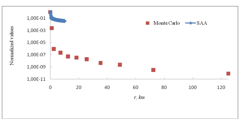
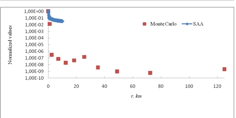
Figures 1-4 present the data for different wavelengths: the SAA calculation (according to formula (11)) of PSF, normalized by h
(
0,30)
(curve 1); and the Monte Carlo calculation of brightness distribution, normalized by I( )
0 (curve 2).Fig. 1. The normalized functions for λ=0.347 µm.
Fig. 2. The normalized functions for λ=0.53 µm.
Fig. 3. The normalized functions for λ=0.69 µm.
Fig. 4. The normalized functions for λ=1,06 µm.
Analysis of data, presented in these figures, makes it possible to draw the following conclusions. The normalized functions are close in value near the direction of radiation from the source ω0 (i.e., for small r) and considerably differ when moving away from this direction (i.e., for large r). Thus, SAA can be used to calculate the point spread function in combination with the Monte Carlo method, in order to reduce the volume of the calculations and time consumptions in the case when large-scale calculations are performed. The usage algorithm may be as follows: 1) calculate hMC
( )
0 by the Monte Carlo method; 2) in small-angle approximation near the direction of radiation from the source ω0, determine PSF hSAA( )
r and normalize it by hSAA( )
0 ; 3) multiply the obtained normalized values by( )
0MC
h ; 4) calculate the point spread function hMC
( )
r by the Monte Carlo method further, for large r.7. CONCLUSIONS
In conclusion, we would like to indicate the following points, which characterize the significance of this work.
1) We obtained and analyzed the results of studying the dependence of the point spread function and optical transfer function on optical-geometrical conditions of observations, which have practical interest in that they make it possible to refine the existing algorithms and construct new ones for predicting and correcting the images.
2) Students who participated in the series of works, including also the given work, gained invaluable experience of scientific activity, which will help them faster adapt to work in scientific-research institutions.
3) Complexes of programs, created in the process of research, are ready software products and can be used (and are being used) for the purposes of teaching new students. They also allow for modifications with the purpose of improving the complex to solve new problems.
REFERENCES
Papoulis A. Systems and transforms with applications in optics. McGraw-Hill Book Company. 1st edition. 1968. – 474 pp.
Zuev V.E., Belov V.V., Veretennikov V.V. System theory in optics of disperse media. – Tomsk: Spektr Publishing IAO SB RAS. 1997. – 402 pp.
Vizilter Yu.V., Zheltov S.Yu., Bondarenko A.V., Ososkov M.V., Morzhin A.V. Image processing and analysis in problems of machine vision: Course of lectures and practical training. – Moscow: Fizmatkniga, 2010. – 672 pp.
Marchuk G.I., Mikhailov G.A., Nazaraliev M.A., Darbinyan N.A., Kargin B.A., Elepov B.S. Monte Carlo method in atmospheric optics. Ed. Marchuk G.I. – Novosibirsk: Nauka, 1976. – 280 pp.
Zege E.P., Ivanov A.P., Katsev I.L. Image transfer in scattering medium. – Minsk: Nauka i tekhnika, 1985. – 327 pp.
Ermakov S.M., Mikhailov G.A. Course of statistical simulation – Moscow: Nauka, 1976. – 320 pp.
Krekov G.M., Rakhimov R.F. Optical-radar model of continental aerosol. Nauka. Novosibirsk. 1982. – 198 pp.
Kvatch A.S. 2013, “Studying the characteristics of radiation from different sources on the basis of the methods of statistical simulation”. Master thesis. National Research Tomsk State University. Tomsk.
Braslavskaya O.B. 2014, “Optical transfer function calculated using small-angle approximation and its application for imaging through the atmosphere”. Master thesis. National Research Tomsk State Uni-versity. Tomsk.