MACHINE LEARNING BASED IMAGE PROCESSING USING UNSUPERVISED APPROACH
Dhanalakshmi Samiappan1, S. Latha2, Deepak Verma3, CSA Sri Harsha4, A. Sashank5
Department of ECE, SRM Institute of Science and Technology, Kattankulathur, Chennai, Tamil Nadu, India. [email protected]
Article received 12.7.2018, Revised 16.8.2018, Accepted 24.8.2018
ABSTRACT
Enhancing the visual media for the purpose of better perception has been a research topic for years. It finds its secondary application in the recognition of objects, analysis of medical images accounting the astronomical data and so on. The disintegration of an image based on its meaningful components plays a key role in many image processing applications like filtering, interpolation, image enhancement, feature variation, etc. the solution to this vary from basic segmentation techniques to advanced methods like fuzzy logic and machine learning. Through this paper, we present a novel method of image processing using machine learning algorithms. We also conduct experiments with preliminary image processing techniques and provide comparable performance measures to illustrate the success of our approach.
Index Terms – Sparse representation, Dictionary Learning, Regularization, Clustering, Unsupervised Learning
I. INTRODUCTION
Image processing as a domain is a vast topic and nonetheless to say that the wide range of appli- cations it provides are worth the research was done in this field. This paper is focused on how the emp- loyment of machine learning approach can simplify the task of image processing both concerning the complexity of processing and quality of output. In this paper, we have used two aspects of machine learning namely regularization and clustering (un-supervised approach [Michael and Bishop 2012]) and some of the basic techniques like bilateral filte- ring [Tomasi and Manduchi, 1998], etc. for comp-aring the performance of our approach. We prima-rily aim at solving the problem of rain removal and secondarily the Gaussian noise. The former being the structured form of noise and latter being the un-structured noise patterns. We have successfully tried to bring out the differences from other meth-ods used and the dominance of our approach over them.
A. Sparse Representation: Sparse modelling
[Olshausen and Field, 1996, Mallat and Zhang, 1993, Bruckstein, and Donoho, 2009] finds its extensive use in the field of image processing appl-ications. Here we employ it for the purpose of image denoising. Image denoising is achieved by minimization of the following energy function:
𝐸(𝐼) =1
2‖𝐼 − 𝐼
′‖ + 𝑅 (𝐼)
Where I’ is a noisy image and I is the required image. R (I) is called the priori or regularization parameter. This method is based on probability. The prior can be modified based on the requirement and hence can be used for efficient modelling of images.
The two basic components of sparse modelling are a dictionary, D (will be discussed in the next section) which consist of atoms and a sparse
coefficient vector β. Atoms are the linear summa-tion of small basis funcsumma-tions which constitute the columns of D. Sparse representation uses the prod- uct of these two to approximate the signal of inter- est I. Consider a dictionary D of dimension N×K. Let K be the size of sparse coefficient vector β with L at the greatest number of non-zero elements of β such that L≪K, the Dβ=I, where I is the image sig-nal of interest. Sparse model of a sigsig-nal is very flexible and abundant in nature as it allows us to use any combination of L atoms from set of K atoms to represent our signal. Sparsity is measured using 𝑙𝑝 norm where we count the number of
non-zeros in β. Empirical results show that most favor-able results are obtained when p lies between 0 and 1, which tends to idealize as p→0.
TABLE I: Performance comparisons (In terms of PSNR-Peak Signal to Noise Ratio, MAE-Mean Arithmetic Error, MSE-Mean Squared Error, RMSE- Root MSE-Mean Squared Error by varying number of atoms)
B. Dictionary Acquisition: Dictionary (refer Fig.
1) learning [Mairal, 2010, 2012, Elad and Aharon, 2006] is a method of training the relevant data such that it most closely summarises the required output.
TABLE II: Performance comparisons (In terms of PSNRPeak Signal to Noise Ratio, MAE-Mean Arithmetic Error, MSE-Mean Squared Error, RMSE- Root MSE-Mean Squared Error)
ALGORITHM PSNR (dB) MAE MSE RMSE
BILATERAL KSVD 37.2911 34.6724 0.0064 0.0086 12.1329 22.1730 3.4832 4.7089
OUR METHOD 41.5319 0.3340 0.1058 0.3253
Performance Measures
1 atom 2 atoms 5 atoms
OMP LAR OMP LAR OMP LAR
Through dictionary learning, we try to reduce the dimensionality of the image from a very high dimension to very low dimensional space and hence it is possible to remove the noise from the image as we are using only a few atoms for the app-roximation of our image of interest. To find the best-fit sparse code and most favourable dictionary we need to eradicate the trivial solutions and find the apt solution to the following equation;
𝐸 = argmin
𝜃𝑝 1
2(‖𝐷𝛽𝑝− 𝐼𝑝‖) + γ‖𝛽𝑝‖1 (2),
where 𝐼𝑝 is the 𝑝𝑡ℎ patch of the image I. Two
itera-tive steps are followed for the optimization of the above equation
1. In the first step I is calculated keeping D unch-anged and,
2. In the second step D is calculated keeping I un-changed.
The above method is iteratively followed until a desired solution is obtained.
Fig. 1: Learnt dictionary; Training time 16.7s, using 65536 patches
Fig. 2: (a) Reference Image (b) Bilateral Filtered Image (c) K-SVD filtered image (d) image filtered using our method
II.FRAMEWORK:BRIEFUNDERSTANDING
A. Finding a sparse solution: In most of the
deno-ising problems using our approach our goal is to
find the sparsest coefficient vector β of 𝑙0 norm
such that it minimizes the mean squared error as
much as possible i.e.‖𝐷𝛽𝑝− 𝐼𝑝‖2 2
≤ 𝜀2 and is uni- que in nature. But the complexity of pseudo-norm makes this task almost unsolvable or solvable with an indefinite amount of time. There are two types of basic approaches that are supported; the first one is called the relaxation method or The Basis Purs-uit. In this method, the penalization factor zero of the pseudo-norm is replaced by one. This results in a convex problem which is solvable in nature at the same time avoid the time constraints. One such approach is least angle regression (LAR) or Stage wise LAR as in [Efron Bradley, 2004].
The second method is called greedy approach or matching pursuit (MP)[MallatandZhang, 1993]. This algorithm iterates by finding one atom at a time. Suppose I' is the image signal we are trying to approximate. The matching pursuit first traver-ses through the columns of the dictionary to look for the atom that is nearest to I'. In the next traver- sal, it searches the atom such that it minimizes the mean square error i.e. ‖𝐷𝛽 − 𝐼′‖
2
2 . It continues to
run until it finds the atoms which minimize the ave- rage squared error below a certain threshold deter-mined by I. In an advanced version of MP the sig-nal I' is projected over the entire set of atoms and an optimal solution is found by the method of least-squares which decreases the time consumption of the algorithm. It is named as Orthogonal Matching Pursuit (OMP).
III.CLUSTERINGANDREGULARIZATION:
ANOVERVIEW
A. Clustering: When the learning is to be done
from a data set that is not labelled or classified it follows an unsupervised learning [Olshausen and Field, 1996] approach as the machine does not have any information about the training data or any prior relation between the noisy image and its denoised version. In such cases learning is achieved by grou-ping of data points or clustering. The data points aresegregatedbasedonsimilar features. Each group or cluster consists of an exemplar which best repre- sents that particular cluster. In our case of image processing clustering algorithms are performed on the atoms. The grouping criteria of atoms is such that they contain same texture and edges is based on a similarity function;
𝑠(𝑎𝑖, 𝑎𝑗) =‖𝐻𝑂𝐺(𝑎𝑖) − 𝐻𝑂𝐺(𝑎𝑗)‖ 2
(3),
where HOG (∙) is Histogram Oriented Gradient
[Bossu, 2011] and describes the shape and context information of the atom. 𝑠(𝑎𝑖, 𝑎𝑗) describes the
similarity between two atoms 𝑎𝑖 and 𝑎𝑗 which is
error. The task of clustering is accomplished by reducing the net similarity, S between the atoms:
𝑆 = ∑𝑀𝑖=1∑𝑀𝑗=1𝑐𝑖𝑗𝑠(𝑎𝑖, 𝑎𝑗) − 𝛾 ∑𝑀𝑖=1(1 −
𝑐𝑖𝑖)( ∑𝑀𝑗=1𝑐𝑖𝑗) − 𝛾∑𝑀𝑖=1|(∑𝑀𝑗=1𝑐𝑖𝑗) − 1| (4)
B. Regularization: In machine learning, the meth-
ods of linear and logistic regression cause the prob-lem of overfitting for high dimensional space. In simple term, the solution to the regression is so acc- urate that it reduces the learning efficiency and inc-reases the complexity. When regularization in imp- lemented on a set of data points, it adds some addi- tional data to the set of data points hence improving the learning performance and reducing complexity. This is accomplished by regularization parameter as in (1). With the large value of γ models with high complexity are made redundant and with a low value of γ training errors are reduced. One such method of regularization is least angle regression. The LAR algorithm help in estimating which atoms to be used to get our response image. It is similar in steps to stepwise regression [Michael and Bishop 2012, Tomasi and Manduchi, 1998] but instead of including atop at every step, the appro-ximated parameters are increased in a direction equiangular to each one's correlations with the residual.
C. Affinity Propagation: When it comes to cluster-
ing, affinity propagation is one of the most suitable algorithms because of its time and error minimi-zation properties. Unlike conventional clustering algorithms like K-means or K-medoids, this appro-ach does not require the number of clusters to be specified before the processing. Not only that this approach provides flexible optimization according to the needs of the user. As mentioned in Frey and Dueck [2007], affinity propagation constantly ach-ieved lower error rate in more than two orders of time when compared to K-means.
Consider a set of random data points from 𝑎1
to 𝑎𝑛 with each point equally potential of
becom-ing an exemplar. Let s be similarity function as mentioned in (3). It represents the similarity or affinity of a point 𝑎𝑖 to point𝑎𝑗. The optimization
parameter or input preference in decided by the diagonal values of s i.e. s (i, i). Input preference should be chosen carefully as it shows the likeli-hood of a point to become exemplar and is an imp- ortant factor in deciding the classes. The algorithm progresses by cycling between two message pass-ing steps to upgrade a couple of matrices namely responsibility matrix R and availability matrix V. 1. The responsibility matrix R measures the
cand-idature of a data point 𝑎𝑘 to become an
exem-plar for 𝑎𝑖 when compared to another point 𝑎𝑗
in the neighborhood of𝑎𝑘.
2. The availability matrix V measures the fitness of 𝑎𝑖 to choose 𝑎𝑘 as its exemplar point when
compared with the preferences of other neighb- orhood points.
In the beginning both the matrices are set to null value and the algorithm progresses through the fol-lowing cyclic steps:
1) Updating of R:𝑟(𝑖, 𝑘) ← 𝑠(𝑖, 𝑘) − max
𝑘′≠𝑘 {𝑎(𝑖, 𝑘
′) +
𝑠(𝑖, 𝑘′)}.
2) Updating of V: 𝑣(𝑖, 𝑘) ← min (0, 𝑟(𝑘, 𝑘) +
∑𝑖′∉{𝑖,𝑘}max (𝑜, 𝑟(𝑖′𝑘))) for i ≠ 𝑘 and v(k,k) ←
∑ max (0, 𝑟(𝑖′, 𝑘))
𝑖′∉{𝑖,𝑘} for i=k.
The above steps are repeated until no more changes occur in the matrices or for some fixed number of iterations.
(a)
(b)
(c)
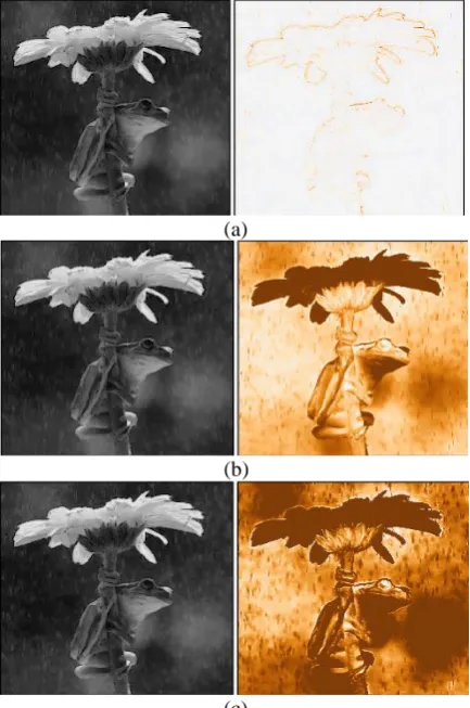
Fig. 3 (a),(b),(c) OMP with 1 atom, 2 atoms and 5 atoms respectively
IV.PROPOSEDMETHOD
1. We take a rainy image (refer Fig. 5), I and perf- orm Discrete Cosine Transform (DCT) to split the image into two components namely high frequency component 𝐼𝐻 and low frequency
component 𝐼𝐿 (refer Fig. 4).
2. From the empirical results we know that most of the structured noise is present in 𝐼𝐻, so we
only take the high frequency component to the next stage while preserving the low frequency component.
3. For edge preservation window filtering is app- lied to the high frequency component.
4. The high frequency component is then given to dictionary learning; Fig. 1 for training the ima-ge data.
5. The next step is to apply a suitable clustering algorithm like affinity propagation [Mallat and
Zhang, 1993] to the atoms of the dictionary to form K clusters of the high frequency compo-nent of the image.
6. Since this method is unsupervised, K is an unk-nown. Once the clusters are formed, process of image reconstruction is done. For K clusters, we get K high frequency image components i.e. 𝐼𝐻1 to𝐼𝐻𝐾.
7. Standard deviation is calculated for these ima-ge components to find the one with least devia-tion from the noisy image since that component will consist. Let it be 𝐼𝐻𝐿
8. Now 𝐼𝐻 is constructed using K-1 components
leaving𝐼𝐻𝐿. Let it be𝐼𝐻′.
9. Finally, to obtain the denoised image 𝐼𝐻′ is
added to its corresponding 𝐼𝐿 to obtain I et al
I=𝐼𝐻′+𝐼𝐿.
Fig. 5: Processing diagram for the proposed method for image denoising and rain removal
V.EXPERIMENTSCONDUCTED
1. First, we have used some basic decomposition and image denoising techniques using bilateral filtering[TomasiandManduchi, 1998], K-SVD [Elad and Aharon, 2006, Aharon, 2006] deco- mposition techniques (refer Fig. 2).
2. Dictionary learning was accomplished by means of LAR and OMP and affinity propaga-tion was used for unsupervised learning. The results are displayed in Fig. 7 and Fig. 3 respec- tively.
3. The output response was tested for variable number of atoms and difference norm was cal-culated and compared. The corresponding res-ults are plotted in Fig. 6
4. Various performance measures like Peak Sig-nal to noise ratio were calculated and compared for different methods as in Table I and II.
Fig. 6 Plot to depict change in norm difference with varying number of atoms
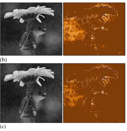
(b)
(c)
Fig. 7a, b and c: LAR with 1 atom, 2 atoms and 5 atoms respectively
VI.CONCLUSION
1. From the results displayed in Table I it is justified that OMP with 1 atom is most suitable for sparse coding of signal.
2. In Table II, though the PSNR values are high compared to OMP and LAR methods, the performance in terms of error is very less and the valuable image features are destroyed which is not desirable.
Thus, using the result displayed in Fig. 2, 3, 6 and 7 and the performance measures tabulated in Table I and II, it is reflected that the machine learning approach to image processing is advanced in terms of time complexity and accuracy. Also, it requires less human effort and is a more intelligent way for advanced signal processing.
VII. REFERENCES
Bruckstein A.M., D.L. Donoho and M. Elad, From sparse solutions of systems of equations to sparse modeling of signals and images. SIAM Rev. 51(1): 34–81 (2009).
Olshausen B.A.and D.J.Field,Emergenceof sim-ple-cell receptive field properties by learning a sparse code for natural images. Nature 381 (13): 607-609 (1996)
Frey B.J. and D. Dueck, Clustering by passing messages between data points. Science 315 (5814): 972-976 (2007).
Tomasi C. and R. Manduchi, Bilateral filtering for gray and color images. Proc. IEEE Int. Confe-rence onComputerVisionPp.839-846 (1998). Efron Bradley, Trevor Hastie, Iain Johnstone and Robert Tribshirani, Least angle regression. Annals of Statistics 32(2): 407-499 (2004). Bossu, J., N. Hautiere and J.P. Tarel, Rain or
snow detection in image sequences through use of a histogram of orientation od streaks. Int.J.Computer Vision 93(3): 348-367 (2011) Mairal, J., F. Bach, J. Ponce and G. Sapiro, Online learning for matrix factorization and sparse coding. J. Machine Learning Res. 11: 19-60 (2010).
Mairal, J., F. Bach and J. Ponce, Task-driven dic-tionary learning. IEEE Trans. Pattern Anal. Mach. Itell. 34(4): 791-804 (2012).
Michael I.J. and C.M. Bishop, Neural networks. Allen B. Tucker, Computer Science Hand bo-ok 2nd Edition (Section VII: Intelligent Syst- ems). Boca Raton, FL: Chapman & Hall/CRC Press LLC ISBN 1-58488-360-360-X (2012). Aharon, M., M. Elad and A.M. Bruckstein, The K-SVD: An algorithm for designing of over complete dictionaries for sparse representat- ion. IEEE Trans. Signal Processing 54(11): 4311-4322 (2006).
Elad M. and M. Aharon, Image denoising via spa-rse and redundant representations over lear-ned dictionaries. IEEE Trans. Image Pro-ces-sing 15(12): 3736-3745 (2006).