DDSC : A Density Differentiated Spatial
Clustering Technique
B. Borah, D.K. Bhattacharyya
Department of Computer Science and Engineering, Tezpur University, Tezpur, India Email:{bgb, dkb}@tezu.ernet.in
Abstract— Finding clusters with widely differing sizes, shapes and densities in presence of noise and outliers is a challenging job. TheDBSCAN is a versatile clustering algorithm that can find clusters with differing sizes and shapes in databases containing noise and outliers. But it cannot find clusters based on difference in densities. We extend theDBSCAN algorithm so that it can also detect clusters that differ in densities. Local densities within a cluster are reasonably homogeneous. Adjacent regions are separated into different clusters if there is significant change in densities. Thus the algorithm attempts to find density based natural clusters that may not be separated by any sparse region. Computational complexity of the algorithm is O(n log n).
Index Terms— Variable density, natural clustering, spatial dataset, noises.
I. INTRODUCTION
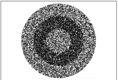
Clustering is one of the most important tasks in data mining and knowledge discovery [1]. The main goal of clustering is to group data objects into clusters such that objects belonging to the same cluster are similar, while those belonging to different ones are dissimilar. By clustering one can identify dense and sparse regions and, therefore, discover overall distribution patterns and interesting correlations among the attributes. Finding clusters in data is challenging when the clusters are of widely differing sizes, shapes and densities and when the data contains noise and outliers. A survey of clustering algorithms can be found in [2]. Although many algorithms exist for finding clusters with different sizes and shapes, there are a few algorithms that can detect clusters with different densities. Basic density based clustering techniques such asDBSCAN [3] andDENCLUE [4] treats clusters as regions of high densities separated by regions of no or low densities. So they are able to suitably handle clusters of different sizes and shapes besides effectively separating noise ( outliers). But they fail to identify clusters with differing densities unless the clusters are separated by sparse regions. For example, in the dataset shown in Fig. 1, DBSCAN finds a single cluster instead of finding the three distinct clusters that can be visualized based on density.
We propose an extension of theDBSCAN algorithm to detect clusters with differing densities. Extracted clusters are non-overlapped spatial regions such that within a region the density is reasonably homogeneous. Adjacent regions are separated into different clusters if
Figure 1. Clusters with varying densities.
there is significant change in densities. The clusters may be contiguous i.e. not separated by any sparse region as required by DBSCAN. Thus natural clusters in a dataset can be extracted. An added advantage is that the sensitivity of the input parameterǫ, which is an important disadvantage of DBSCAN, is reduced significantly. A preliminary work on this algorithm was presented in [5]. Rest of the paper is organized as follows. Related works on density based clustering techniques that can find clusters based on density difference is briefly discussed on section II. Section III provides an introduction to the basic density based clustering algorithmDBSCAN. Our proposed algorithm is presented in section IV. Experimental results in section V shows the effectiveness of the proposed algorithm. Finally, section VI presents a conclusion and direction for future works.
II. RELATED WORKS
To find clusters that are naturally present in a dataset very different local densities need to be identified and separated into clusters. The OP T ICS [6] algorithm adopts DBSCAN to achieve this goal. The proposed algorithm also extendsDBSCAN in a different manner to achieve the same goal. OP T ICS computes an ordering of the objects augmented by reachability distance, representing the intrinsic hierarchical clustering structure. This cluster ordering, displayed by the so called reachability-plots, is the basis for both automatic and interactive cluster analysis. Valleys in this plot indicate clusters. The parameter ξ is crucial for identifying the valleys as ξ-clusters.
DENCLUE (DENsity CLUstEring) [4] takes a more formal approach to density based clustering by modeling the overall density of a set of objects as the sum of influence functions associated with each object. The resulting overall density function will have local peaks, i.e., local density maxima, and these local peaks can be used to define clusters in a straightforward way. Specifically, for each data object, a hill climbing procedure finds the nearest peak associated with that object, and the set of all data objects associated with a particular peak (called a local density attractor) becomes a (center-defined) cluster. However, if the density at a local peak is too low, then the objects in the associated clusters are classified as noise and discarded. Also, if a local peak can be connected to a second local peak by a path of data objects, and the density at each object on the path is above a minimum density threshold, ξ, then the clusters associated with these local peaks are merged. Thus, clusters of any shape can be discovered. It has trouble with data that contains clusters of widely different densities.
In CHAM ELEON [7] and SNN [8] algorithms attempts to obtain clusters with variable sizes, shapes and densities based on k-nearest neighbour graphs. CHAM ELEON finds the clusters in a dataset by using a two-phase algorithm. In the first phase it generates a k-nearest neighbour graph that contains links between a point and itsk-nearest neighbours. This approach reduces the influence of noise and outliers and provides an automatic adjustment for differences in densities. Then it uses a graph partitioning algorithm to cluster the data items into a large number of relatively small subclusters. During the second phase, it uses an agglomerative hierarchical clustering algorithm to find the genuine clusters by repeatedly combining subclusters. No cluster can contain less than a user specified number of instances. It has problems when the partitioning process does not produce subclusters.
The SNN ( Shared Nearest Neighbour) clustering algorithm uses k-nearest neighbour approach to density estimation. It constructs a k-nearest neighbour graph in which each data object corresponds to a node which is connected to the nodes of the k-nearest neighbours of that data object. From the k-nearest neighbour graph a shared nearest neighbour graph is constructed, in which
edges exist only between data objects that have each other in their nearest neighbour lists. A weight is assigned to each edge based on the number and ordering of shared neighbours. Clusters are obtained by removing all edges from the shared nearest neighbour graph that have a weight below a certain threshold τ. SNN can detect clusters of different sizes, shapes and densities.
The clustering techniques stated above try to find clusters with variable sizes, shapes and densities. The proposed algorithm is an alternative to these algorithms. It is simpler and produces good quality results consuming less execution time. For example OP T ICS produces an ordering of the objects by performingk-NN queries in the first step and then it produces variable density clusters using a second step requiring more execution time. DENCLUE and SNN use several parameters, proper tuning of the parameter values is very important for getting good quality results.
III. INTRODUCTION TODBSCAN
Objects in the given datasetD is treated as points in a d-dimensional space Rd. The distance function between two pointsp and q is denoted by dist(p, q). The basic ideas of DBSCAN clustering involve a number of definitions, which are produced below.
• Theǫ-neighbourhood of a pointp, denoted byNǫ(p), is defined asNǫ(p) ={q∈D|dist(p, q)≤ǫ}.
• If theǫ-neighbourhood of a point contains at least minimum number,M inP tsof points, then the point is called a core point i.e. a point p is core if |Nǫ(p)| ≥M inP ts.
• A pointpis directly density reachable from a point q with respect to ǫ andM inP ts if p∈Nǫ(q) and Nǫ(q)≥M inP ts.
• A pointp is density-reachable from a pointq with respect toǫandM inP tsif there is a chain of points p1, . . . , pn,p1=q,pn=psuch thatpi+1is directly density-reachable frompi.
• A point p is density-connected to a point q with respect to ǫand M inP tsif there is a pointo such that both,pandqare density reachable fromowith respect toǫandM inP ts.
• Let D be a database of points. A cluster C with respect toǫ andM inP tsis a non-empty subset of D satisfying the following conditions :
1) ∀p, q:ifp∈Candqis density-reachable from pwith respect toǫ andM inP ts, thenq∈C. (Maximality).
2) ∀p, q ∈ C : p is density-connected to q with respect to ǫandM inP ts(Connectivity).
• LetC1, . . . , Ck be the clusters of the datasetD with respect to parametersǫiandM inP tsi, i= 1, . . . , k. Then noise is defined as the set of points in the database D not belonging to any cluster Ci i.e. noise={p∈D| ∀i : p /∈Ci}.
Given a dataset, ǫ andM inP tsas input, DBSCAN searches for clusters by checking theǫ-neighbourhood of each object in the dataset. If the ǫ-neighbourhood of an objectpcontains more thanM inP ts, a new cluster with p as core object is created. DBSCAN then iteratively collects directly density-reachable objects from these core objects. The process terminates when no new objects can be added to any cluster.
IV. PROPOSEDALGORITHM
The proposed algorithm partitions given dataset into a set of spatial regions (clusters) such that adjacent regions significantly differ in density. Lesser amount of local density variations exist within a cluster, but going from the present region to a neighbouring region greater amount of local density variation will be noticed.
Let, the given numeric dataset, D, consisting of n d-dimensional objects be represented by xij, i = 1. . . n, j = 1. . . d. The p-th object {xp1, xp2, . . . , xpd} can be referred by its serial number p alone. The neighbourhood within a given radiusǫofpis represented by Ne(p) = {q ∈ D|dist(p, q) ≤ ǫ}. It is spherically shaped for Euclidean distance function dist(p, q). The neighbourhood size of an objectpi.e.|Nǫ(p)|represents the density around it. Let us use a list wp, p = 1. . . n to store density of each object in the datasetD. Initially, density of each object is unknown, which is represented by wp = −1, p = 1. . . n. When neighbourhood query is performed, density of p is assigned aswp =|Nǫ(p)|. Object p is called a core object if wp ≥ M inP ts. The dataset is to be partitioned into a set of non-overlapped clusters. Let us denote the cluster label ofpbycp. Initially all objects are assigned the label -1 to indicate unlabeled objects, that iscp=−1, ∀p∈ {1. . . n}.
The algorithm starts a cluster with a homogeneous core object and goes on expanding it by including other directly density reachable homogeneous core objects until non homogeneous core objects, that indicate wide variation in densities, are detected. For detection of clusters separated by density variations the concepts of processed objects, candidate objects, unprocessed objects and homogeneous core objects are required. The definitions are presented below.
• A processed objectpis one, whose density is already evaluated, i.e. wp ≥1. Evaluating the density of an object by performing neighbourhood query is called processing.
• A candidate object is already included in a cluster, but its density is yet to be evaluated, i.e.cp≥0and wp=−1.
• An unprocessed object p has wp = −1, cp = −1, that is its density as well as cluster label are not evaluated.
• A homogeneous core objectpis a core object (wp≥ M inP ts) whose density is neither more nor less than αtimes the density of any of its neighbours. That is ∀q∈Nǫ(p),wp/wq ≤αifwp≥wq orwq/wp≤α if wp < wq whereα >1 is a constant.
An ordering is imposed upon the sequence in which the objects will be processed while expanding a cluster.
A. Ordered Expansion Process
A new cluster is created with the objects found in the neighbourhood of a homogeneous core object detected. This initial cluster is expanded when each object of the cluster is processed and they contribute some new members to be processed later. Unprocessed members wait in a seed list to be processed next. The seed list is denoted byS. Objects are deleted from the front end of the seed list for processing while new members are entered at the back end. When an object is processed it may contribute more than one new objects to the seed list. An ordering is imposed on those new objects for entering into the seed list. The following are the steps for processing an objectptaken out from the seed list.
1) Find the neighbourhood,Nǫ(p); 2) Set the density value,wp=|Nǫ(p)|;
3) Ifpis a homogeneous core perform steps 4-7; 4) Find the list Lp of unlabeled objects in Nǫ(p) :
Lp={q|q∈Nǫ(p), cp=−1};
5) Arrange the objects in Lp in ascending order of their distance to p giving the sorted list Lp with sizet=|Lp|, that is :
Lp = {qi | qi ∈ Lp, i ∈ 1. . . t, q0 = p, dist(qi−1, p)≤dist(qi, p)};
6) AppendLp in seed listS;
7) Mark all unlabeled and noise objects inNǫ(p)with present cluster labelc:
∀q{q∈Nǫ(p), cp≤0}:cp=c;
Steps 4-5 imposes an ordering on the seeds for entering into the seed list. Steps 6-7 expands the cluster. Each object in D is processed serially ( by performing steps 1-3 ) until the first homogeneous core objectois found. Theno is marked with a new cluster label and steps 4-7 are performed for o. Thus the initial cluster with the initial seed list is created. This cluster is expanded by processing each object of the seed list using steps 1-7 until the list becomes empty. The procedure is repeated for finding other clusters in the dataset.
This ordered expansion process has some important properties as presented in the lemmas to follow. In DBSCAN, unlabeled neighbours are inserted into the seed list in the order in which they are obtained. So already processed objects and candidate objects ( waiting in the seed list to be processed ) are intermixed in the same spatial region. By spatial region we mean the region formed when the d-dimensional objects are considered as points in ad-dimensional space. In the discussions to follow we consider 2-dimensional objects for simplicity in graphical presentation, the ideas are applicable to higher dimensions as well. The word spatial may be omitted.
Lemma 1: During ordered expansion process, already
Proof : When a cluster is first created by processing a core objecto, all its neighbours inside the circle of radius ǫbecome candidates to be processed next. Presently, there is only a single objectoin the region of already processed objects, which is surrounded by the region formed by candidate objects. The region of already processed objects grows as candidates become processed and contribute some new candidates. Consider that the next object to be processed currently is p. Let, q be the object which has contributed pto the seed list i.e.p∈Nǫ(q) andqis already processed. Let,s=dist(p, q). Draw a circle with radius s centered at q. All objects inside the circle will be already processed objects. Because, according to the ordered expansion process, all objects rinside the circle will be processed beforep, sincedist(r, q)< dist(p, q). This contiguous region of already processed objects grows by one object after including the currently processed objectp, which lie on the circle. So, the region will still remain contiguous after inclusion of the objectp.2
At least one processed object is present in the neighbourhood of currently processed object. There is a maximum limit for the number of processed objects that may be present in the neighbourhood of currently processed object.
Lemma 2: For uniformly distributed objects at most
50% neighbours in the neighbourhood of the currently processed object are already processed.
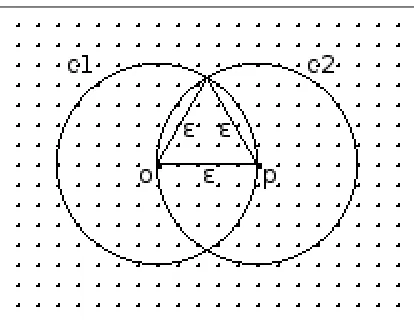
Proof : Consider thatois the first core object detected for expanding a cluster. Ordered expansion procedure processes the objects one by one starting from the nearest neighbour of o, initial few objects have less than 50% already processed objects in their neighbourhoods at the time of processing them. Let the currently processed object p, lying on the circle c1 with radius ǫ centered at o as shown in Fig. 2, be the farthest object in the neighbourhood of object o. The neighbourhood of p is shown by circle c2. The area of intersection of the two circles (Nǫ(o)∩Nǫ(p)) contains already processed objects. Using the formula for circular segment1, the
area of intersection [9] of the two circles is calculated to be 39% of the area of circle c2. Assuming uniform distribution of objects and m = |Nǫ(p)|, this region will contain 0.39m objects. Here, pis selected such that the present region of already processed objects is small enough to be included inside the circle of radiusǫ. But as the cluster grows the region of already processed objects grows in size. Then the already processed objects and candidate objects in the neighbourhood of the currently processed object can be separated with an arc of a circle of larger radius. When the cluster becomes bigger this boundary can be a straight line, in which case 50% of the neighbourhood of the currently processed object will be already processed. 2
Proposed algorithm does not require that objects are uniformly distributed. It detects clusters that are reasonably homogeneous i.e. some amount of density
1A(R, d) =R2cos−1(d/R)−d√(R2−d2),Ris the radius,dis
distance of the segment from the center
Figure 2. Already processed objects within the neighbourhood of currently processed objectp.
variation is allowed within a cluster. Significant variation of density will cause separate clusters to be identified. Lemma 1 & 2 provide us an approach for detecting density variations while a cluster is being expanded. The density of each of the already processed object is known as its density value was stored at the time of processing it. So, we can ensure that the density of the current object processed should not differ much with those of already processed objects in its neighbourhood, otherwise this current object should not be expanded i.e. previously unclustered objects found in its neighbourhood should not be added to the seed list. Below we formalize this homogeneity test.
B. Homogeneity Test
Let,pbe the current object being processed andLpbe the list of already processed objects (wp ≥1, ∀p∈Lp) present in the neighbourhood ofp. The current objectpis homogeneous to the region of already processed objects if the following conditions hold for eachq∈Lp :
wp
wq > α1 if wq ≥wp (1) wq
wp > α2 if wq < wp (2) In the inequalities ( 1) and ( 2) α1, α2 ∈ (0,1] are two constants indicating allowed density difference limits within the neighbourhood of an object. The values ofα1 andα2can be determined based upon an input parameter αas described below.
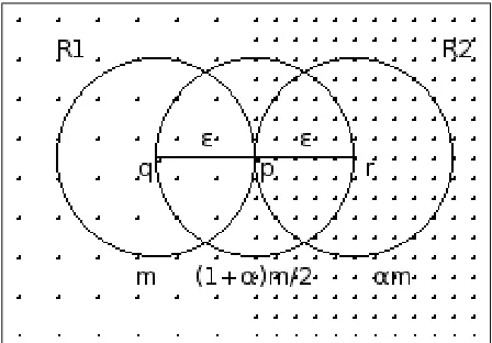
Let us consider two contiguous uniformly distributed regionsR1andR2 as show in Fig. 3, such thatR2 isα times denser thanR1, withα >1. The minimum density difference required for separating clusters is indicated by α. If the density difference is less thanα, the two regions will be merged into a single cluster. Assume that the current object to be processed,pis located at the boundary of the two regions. Consider two objects q ∈ R1 and r∈R2 such thatdist(p, q) =dist(p, r) =ǫ andp,q,r are in a straight line. Let,wq=|Nǫ(q)|=m. Then,wr= |Nǫ(r)|=αm, andwp =|Nǫ(p)|= (1+α)m
Figure 3. Density variation pattern produced by two adjacent regions with different densities.
any object betweenqandpwill be higher thanmbut less than(1+α)m2. Similarly, density of each object betweenp andrwill be higher than(1+α)m2 but less thanαm. So, the objects betweenqandrform a transition ( bordering ) region containing objects with different densities. When a transition region is encountered cluster expansion in that direction may get stopped. A transition region may be encountered while going from a lower density region to a higher density one or from a higher density region to a lower density one. So, two different density factorsα1 andα2 are needed to avoid order dependency. Values of the two factors can be computed based on objectp. While expanding a cluster, if a lower density region is entered, the density difference limit between the density of the current object with any of the already processed objects in its neighbourhood,α1is computed as :
α1=wwp r =
(1 +α)m
2
αm =
1 +α
2α (3)
Similarly, entering a higher density region, the density difference limitα2 is computed as :
α2=wwq p =
m (1 +α)m
2
= 1 +2α (4)
The two factors α1 and α2 determines the allowed variation in local density within a cluster so that the density of the cluster can be called relatively homogeneous.
Above, we have stated about the maximum density difference allowed for a single object to be called homogeneous to the region of already processed objects. To stop growth of a cluster in any spatial direction a non homogeneous region of width at least ǫ should be encountered in that direction. The following lemma establishes the idea.
Lemma 3: The growth of a cluster in any spatial
direction is stopped if a non homogeneous region of width at least αis encountered in that direction.
Proof : Referring back to Fig. 3, object p is the current object being processed. Object p becomes non homogeneous, if in the neighbourhood of p there is at least one already processed object that crosses the allowed density variation limit. Let, the region Nǫ(q)∩Nǫ(p)
contain processed objects and wq/wp < α2, causing objectp to become non homogeneous. Then pwill not be expanded but growth of present cluster can not be stopped bypalone. Since, there are some candidates for expanding the cluster lying afterpand those candidates were contributed by the objects present between q and p when they were processed. These candidate objects form a region of width at most ǫ, that is spread up to just before objectr. To stop growth of the cluster in the direction ofq tor, none of these objects should expand when processed. That is, each of these objects should become non homogeneous because of presence of some predecessors, lying between q and p, that have density difference greater than allowed limit. This will really be the case if the region betweenq and r (region R2 ) is denser than the region betweenq andp(regionR1 ) by a factor greater thanα.2
From lemma 3 it becomes clear that a cluster extends beyond its expected boundary as some non homogeneous objects ( border objects ) are also included in the cluster. It is because we are performing homogeneity test only on one part of the neighbourhood. We cannot test the remaining part simultaneously because density information of these objects will be obtained only when they are processed. Another problem is that the region of already processed objects falling in the neighbourhood of currently processed object may contain very few objects that may lead to single linkage effect. To alleviate these two problems we impose the following requirements on the currently processed object. We call it cardinality test.
C. Cardinality Test
The number of already processed objects present in the neighbourhood of currently processed object should be within a certain minimum and maximum limits. The maximum limit is taken to be 50% of the neighbourhood size based on lemma 2. The volume of intersection of two d-dimensional hyper spheres with radius ǫ situated at a distance of ǫ apart gives the minimum limit for d-dimensional data objects. The situation is shown for 2-dimensional data in Fig. 2. The area of intersection for two circles is approximately 39% of the area of a circle. For a sphere this is approximately 31% [9]. As the dimension increases this volume decreases. We take the minimum limit to be 1+1d%, where d is the dimension of the data objects. Consider currently processed objectp in Fig. 3. Proceeding from q top i.e. going from lower to higher density, minimum possible number of already processed objects contained in the neighbourhood ofpare
m
1+d. Similarly, proceeding from r to p i.e. going from higher to lower density, maximum possible number of already processed objects contained in the neighbourhood ofpare αm2 . So, the two limits expressed as a fraction to the density of the currently processed object are
βmin=(1 +1+mαd)m
2
βmax= αm2
(1 +α)m
2 =
α
1 +α (6)
D. Spatial treatment for the First Core Object
The homogeneity test and cardinality test are not applicable to the starting core object of the cluster, as no objects of the cluster are processed before it. However, it must be ensured that the first object does not lie at the boundary of two widely differing density regions. In fact, it must not lie within a distance of ǫ/2 from the boundary. Otherwise the two differing density regions will be merged into a single cluster. Because, a non homogeneous region of width at least ǫ will not be encountered in that case to stop the growth of the cluster across the boundary as required by lemma 3.
To avoid this problem we reject the outer neighbours of the first core object and enter into the seed list only those neighbours that lie within a radius of ǫ/2 from the object. Cardinality test is also not applied while these few seeds are expanded.
E. The Algorithm
The steps in DDSC clustering algorithm is presented below.
1) input ǫ, M inP ts, α, D;
2) initialize all objects in D as unlabeled and unprocessed;
3) Compute :
α1= (1 +α)/(2∗α); α2= 2/(1 +α);
βmin= 2/((1 +d)∗(1 +α)); βmax=α/(1 +α);
4) repeat steps 5-7 until all objects inDare clustered; 5) examine each object and begin a new cluster with a core object; Apply special treatment for the first core object;
6) expand the cluster using ordered expansion process; 7) apply the homogeneity test and cardinality test
during expansion; 8) end;
F. Complexity Analysis
The most time consuming part of the algorithm is the neighbourhood queries. The neighbourhood size is expected to be small compared to the size of the dataset. So, the different tests performed on the neighbourhood will not consume much time. While expanding a cluster the list of newly contributed seeds by each object of the cluster need to be sorted. For all objects only a small fraction of the neighbours become new seeds, whereas some objects contribute no new seeds at all. Sorting the lists will not consume much time as the size of the list to be sorted is small. The time required for a neighbourhood query is O(log n)by using a spatial access method such as R*-tree. Neighbourhood query is performed for each of the n objects in the dataset. So the run time complexity isO(n log n).
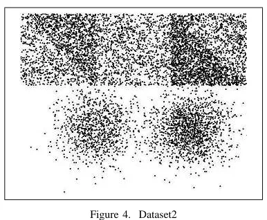
Figure 4. Dataset2
V. EXPERIMENTALRESULTS
In this section we evaluate the performance of the DDSC and compare the result with CHAM ELEON andSNN algorithms. We implemented the algorithm in C++. Experiments were conducted on a 1.66 GHz HCL laptop with core dual processor, 512 MB RAM running LINUX operating system.
Synthetic datasets are used in the experiments. The CHAM ELEON datasets - t4.8k.dat, t7.10k.dat, t8.8k.dat and t5.8k.dat, used in [7] are downloaded from [10]. We have created two dataset -Dataset1shown in Fig. 1 and Dataset2 shown in Fig. 4. Dataset1 contains 24000 objects arranged in three nested circular regions, the middle region being twice as much denser than the neighbouring ones. Dataset2 contains 8100 objects. Four triangular regions and a rectangular region are generated such that a region is at least two times denser than the neighbouring regions. These can be visualized in the upper part of the figure. Local density variations are present within each region. Two regions are produced using Gaussian density generator.
The clustering results forDataset1andDataset2are shown in Fig. 5 and Fig. 6. Different colours are used to indicate the clusters. It can be seen from the figures that the circular, triangular and rectangular clusters are extracted based on differences in densities although they are not separated by sparse regions. The three nested clusters with different densities inDataset1are properly extracted. Bigger portions of the Gaussian clusters in Dataset2 are also detected, which means that inside a cluster the local densities may gradually change within limits, bigger changes prevents the expansion of the clusters.
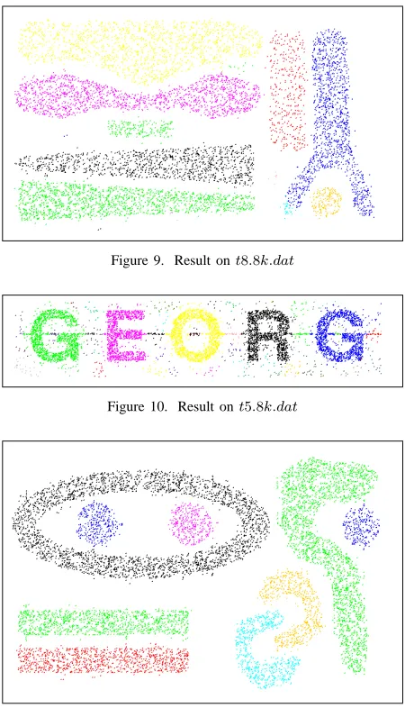
Figs. 7- 10 show clustering result of our algorithm on CHAM ELEON datasets - t4.8k.dat, t7.10k.dat, t8.8k.dat and t5.8k.dat respectively. Clusters with different sizes, shapes and densities are extracted and noises are discarded. Similar results were reported for CHAM ELEON [7] andSNN [8] algorithms.
A. Discussion on Parameters
Figure 5. Result onDataset1
Figure 6. Result onDataset2
Figure 7. Result ont4.8k.dat
Figure 8. Result ont7.10k.dat
Figure 9. Result ont8.8k.dat
Figure 10. Result ont5.8k.dat
Figure 11. Result on t7.10k.dat with increasedM inP ts
B. Order Dependency
We have repeated the above mentioned experiments several times, each time the objects of the dataset are shuffled randomly. The results produced the same set of clusters except changes in cluster memberships of a few bordering objects. It means that the algorithm is not very much order dependent.
All these results show that our algorithm can find clusters with variable sizes, shapes, and densities. Noises are also properly separated.
VI. CONCLUSION
In this paper we have presented DDSC algorithm that provide a solution for the problem of finding clusters with varying sizes, shapes and densities. Clusters extracted from a dataset are non-overlapped spatial regions having different densities. Adjacent clusters may be very close, without being separated by any sparse regions. The algorithm is an extension of DBSCAN and uses a homogeneity test to detect density variations. A cluster is reasonably homogeneous locally. It uses a parameter αto indicate allowed density variation within a cluster besides using the parameter ǫ and M inP ts. Non homogeneous regions indicate cluster boundaries. The time complexity of the algorithm remainsO(nlog n). It also alleviates another important disadvantage of DBSCAN - sensitivity of input parameter ǫ. In our algorithm,ǫcan vary in an wide range without any change in the clustering result.
The experiments were done using 2-dimensional data sets only. In future works performance of the algorithm may be evaluated on medium and high dimensional datasets. Some modifications may be needed to handle inherent sparseness of high dimensional data. In high dimensional data all the dimensions may not be equally important for determining cluster membership of an object, which is another aspect to be dealt with.
REFERENCES
[1] J. Han and M. Kamber, Data Mining Concepts and Techniques. Morgan Kaufman, 2006.
[2] R. Xu, “Survey of Clustering Algorithms,” IEEE
Transaction on Neural Networks, vol. 16, no. 3, May 2005. [3] M. Ester, H. P. Kriegel, J. Sander, and X. Xu, “A density-based algorithm for discovering clusters in large spatial data sets with noise,” in 2nd International Conference on Knowledge Discovery and Data Mining, 1996, pp. 226– 231.
[4] A. Hinneburg and D. Keim, “An efficient approach to clustering in large multimedia data sets with noise,” in 4th International Conference on Knowledge Discovery and Data Mining, 1998, pp. 58–65.
[5] B. Borah and D. K. Bhattacharyya, “A clustering technique using density difference,” in Proceedings of International Conference on Signal Processing, Communications and Networking(ICSCN-2007), Mar. 2007, pp. 585–588. [6] M. Ankerst, M. Breunig, H. P. Kriegel, and J. Sander,
“OPTICS: Ordering Objects to Identify the Clustering
Structure, Proc. ACM SIGMOD,” in International
Conference on Management of Data, 1999, pp. 49–60.
[7] G. Karypis, E. H. Han, and V. Kumar, “CHAMELEON:
A hierarchical clustering algorithm using dynamic
modeling,” Computer, vol. 32, no. 8, pp. 68–75, 1999. [8] L. Ertoz, M. Steinbach, and V. Kumar, “Finding clusters
of different sizes, shapes, and densities in noisy, high dimensional data,” in Proceedings of Second SIAM International Conference on Data Mining, Jan. 2003.
[9] E. W. Weisstein, “Sphere-Sphere Intersection,”
from MathWorld – A Wolfram Web Resource.
http://www.mathworld.wolarm.com/Circle-CircleIntersecton.html.
[10] Http://www.glaros.dtc.umn.edu/gkhome/cluto/cluto/down-load.
B. Borah is currently a lecturer of Computer Science and
Engineering at Tezpur University, Tezpur, India. He received his MS degree in Systems and Information from Birla Institute of Technology and Science, Pilani, India in 1997. He is also a Ph.D. research scholar at Tezpur University, Tezpur, India. His research interests include Data mining, Pattern Recognition and Image Analysis.
D. K. Bhattacharyya is currently a Professor of Computer