Evaluation Of Walficsh-bertoni Path Loss Model Tuning Methods For A Cellular Network In A Timber Market In Uyo

(1)

Evaluation of Walficsh-Bertoni Path Loss

Model Tuning Methods for a Cellular Network in

a Timber Market in Uyo

Kalu Constance1, Ozuomba Simeon2 , Umana, Sylvester. Isreal 3, 1,2,3

Department of Electrical/Electronic and Computer Engineering, University of Uyo, Akwa Ibom, Nigeria *Corresponding Author: [email protected]

Abstract— In this paper, an evaluation of four different Walficsh-Bertoni path loss model tuning methods for a cellular network in a timber market located on the outskirts of Uyo in Akwa Ibom state is presented. The study used empirically measured signal strength intensity data obtained within the market for a 1800GHz 3G cellular network to compare the prediction performance of the different model optimization methods. Particularly, the received signal strength intensity, the transmitting base station information and other relevant information required for the study are collected with the use of G-NetTrack Lite 8.0 wireless network site surveying android app installed on Samsung Galaxy S8 phone. The four tuning methods considered are the root mean square (RMSE)-based tuning, the coefficient of the path length-based tuning, the coefficient of the logarithm of the path length-based tuning, the composition function of residue-based tuning. The results show that the composition function-tuned Walficsh-Bertoni model has the best prediction performance with the least RMSE of 1.5 dB, least MAPE of 1.2 dB and the highest prediction accuracy of 99.1%. It also maintained the best prediction performance with the validation dataset. The coefficient of the path length-based method is the second, followed by the popular RMSE-tuned Walficsh-Bertoni model. In all, this paper has demonstrated that while the RMSE method is popular, there are other simple tuning methods that can perform better.

Keywords— Path Loss, Path Loss Model, Semi-Empirical Path Loss Model, Cellular Network, Walficsh-Bertoni Model.

I. INTRODUCTION

Accurate prediction of the expected path loss is essential in wireless network system planning [1,2,3,4,5,6]. As such, several analytical expressions have been developed over the years for estimating the path loss that wireless signals will experience when propagating through a given environment [7,8,9,10,11,12,13]. The path loss models are classified as empirical, semi-empirical and deterministic models [14,15,16,17]. Among the three

models are more popular. However, the semi-empirical models are particularly useful for combining some site-specific features and empirical measurements in determining the expected path loss in the given environment [18,19,20,21,22].

In all, studies have shown that no single path loss model can fit all environments [23,24,25,26,27,28,29]. Rather, the models are optimized for any given environment based on field measurements conducted within the environment of interest. Accordingly, in this paper, an empirical field measure path loss data is used to optimize Walficsh-Bertoni model [30,31,32,33,34] for a timber market. The choice of Walficsh-Bertoni model is particularly important as it is a semi-empirical model includes the building height and the space between buildings as part of the parameters it uses to estimate the path loss in a given environment. The case study timber market has rows of buildings for the timber shops along with a series of frames for hold timbers in front of the timber shops.

More importantly, the focus of this paper is to examine the effectiveness of different Walficsh-Bertoni model optimization methods. The essence of the study is to present different methods that can be used to obtain better path loss prediction accuracy than the popularly used root mean square error (RMSE) based model optimization approach. Accordingly, four different optimization methods are considered and their prediction accuracy is examined in respect of the RMSE, the prediction accuracy and maximum absolute prediction error. The relevant mathematical expressions and model development and evaluation procedures are presented.

II. THE WALFICSH-BERTONI PATH LOSS MODEL

Among the various semi-empirical path loss models, the Walficsh-Bertoni model is particularly suitable for characterizing path loss in an area with much building obstruction in the signal path.The Walfisch-Bertoni model is expressed as [30,31,32,33,34];

𝑃_𝑊𝐵(𝑑𝐵) = 89.5 − 10 (log10( 𝜌1𝑅0.9

(𝐻𝐵−ℎ𝑚)2)) +

21(log₁₀(𝑓𝑚)) − 18(log10(ℎ𝑏− 𝐻𝐵)) + 38(log10(𝑑)) (1) Where;

𝜌1= √(( 𝑅

(2)

Vol. 4 Issue 12, December - 2018 ℎ_𝑏 is the transmitter antenna height in meters; R:

Space between buildings in meters; 𝐻𝐵 is the building height in meters, 𝑓_𝑚 is the frequency in MHz; ℎ_𝑚 is the mobile height in meters and d: is the distance between base station transmitter and the mobile station in Km.

III. THE EMPIRICAL DATA COLLECTION

The field measurement is carried out along within a timber market on the outskirts of Uyo. market lies within the signal coverage area of a 1800GHz 3G cellular network. The buildings in the timber market are about 5 meters high with an average distance of 6 meters between the buildings. The received signal strength intensity (RSSI), the transmitting base station information and other relevant information required for the study are collected with the use of G-NetTrack Lite 8.0 wireless network site surveying android app installed on Samsung Galaxy S8 phone. The field measurement was conducted in November 2018. The RSSI data was used to compute measured path loss. The entire measured path loss dataset was divided into two parts and a part was used for the model training while the other part was used for validating the optimized models developed in this paper. The measured path loss are versus path length are shown in Figure 1 for the training and the validation datasets.

Figure 1 The measure path loss are versus path length for the training and the validation

datasets

The prediction performance of the model is evaluated using the root mean square error (RMSE) , prediction accuracy (PA) and maximum absolute prediction error (MAPE) where;

RMSE = √{ 1

𝑛[∑ | 𝑃𝑚(𝑖)− 𝑃𝑊𝐵(𝑖)| 2 𝑖 = 𝑛

𝑖 = 1 ]}

2

(3) 𝐏𝐀 = (1 − (1

𝑛 (∑ |

𝑃𝑚(𝑖)−𝑃𝑊𝐵(𝑖)

𝑃𝑚(𝑖) |

𝑖=𝑛

𝑖=1 ))) * 100 %

(4) MAPE = maximum(| 𝑃_𝑚(𝑖)− 𝑃_{𝑊𝐵(𝑖)}| for all i ≥)1

(5) Where 𝑃_𝑚(𝑖) is the measured path loss at data point i

and𝑃𝑊𝐵(𝑖) is the Walficsh-Bertoni model path loss prediction for data point i.

IV OPTIMISATION OF THE WALFICSH-BERTONI MODEL

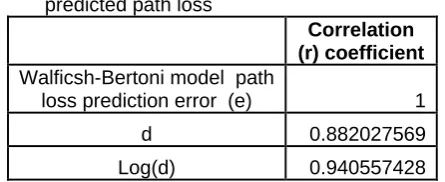
In order to select the parameters to be adjusted for the model tuning, the correlation between the Walficsh-Bertoni model path loss prediction error and

three other parameters were determined as shown in Table 1

Table 1 The correlation between the Walficsh-Bertoni model path loss prediction error and three other parameters (path length, log of the path length and the Walficsh-Bertoni model predicted path loss

Correlation (r) coefficient Walficsh-Bertoni model path

loss prediction error (e) 1

d 0.882027569

Log(d) 0.940557428

The result showed very strong correlation between the error, e and Log(d) followed y the correlation between the error, e and d. Consequently, the model prediction error can be effectively reduced by a tuning method that adjust the coefficient of d, or the coefficient of Log(d). Also, a composite function that estimates prediction error as a function of the distance, d will also provide good result. As such, four tuning approaches or options are considered.

(I) The RMSE-based tuning approach

This is the common path loss model tuning technique and for the case study path loss model it is given as;

𝑃_{𝑊𝐵_𝑅𝑀𝑆𝐸(𝑖)}=

{𝑃𝑊𝐵(𝑖)+ 𝑅𝑀𝑆𝐸 𝑓𝑜𝑟 ∑( 𝑃𝑚(𝑖)− 𝑃𝑊𝐵(𝑖)) ≥ 0 𝑃_{𝑊𝐵(𝑖)}− 𝑅𝑀𝑆𝐸 𝑓𝑜𝑟 ∑( 𝑃_𝑚(𝑖)− 𝑃_{𝑊𝐵(𝑖)}) < 0 (6) The RMSE is determined from the field measured path loss and the Walficsh-Bertoni model predicted path loss values.

(II) The coefficient of d-based tuning, denoted as (CD-tuning ) is given as

𝑃_{𝑊𝐵_𝐶𝐷(𝑖)}= 89.5 − 10 (log₁₀( 𝜌1𝑅0.9

(𝐻𝐵−ℎ𝑚)2)) +

21(log₁₀(𝑓𝑚)) − 18(log10(ℎ𝑏− 𝐻𝐵)) + 38(log₁₀(𝐾_𝐶𝐷(𝑑))) (7) Where K_CD is the coefficient of d that is adjusted until the minimum RMSE value is realized. The value of 𝐾_𝐶𝐷 is determined from the field measured path loss and the Walficsh-Bertoni model predicted path loss values.

(III) The coefficient of Log(d)-based tuning, denoted as (CLD-tuning ) is given as

𝑃𝑊𝐵_𝐶𝐿𝐷(𝑖)= 89.5 − 10 (log10( 𝜌1𝑅

0.9

(𝐻𝐵−ℎ𝑚)2)) +

21(log10(𝑓𝑚)) − 18(log10(ℎ𝑏− 𝐻𝐵)) + 38(𝐾_𝐶𝐿𝐷)(log10(𝑑)) (8) Where 𝐾_𝐶𝐿𝐷 is the coefficient of Log(d) that is adjusted until the minimum RMSE value is realized. The value of 𝐾𝐶𝐿𝐷 is determined from the field measured path loss and the Walficsh-Bertoni model predicted path loss values.

120 124 128 132 136 140 144

0.65 0.7 0.75 0.8

P

ath

Loss

(dB)

Path Length , d (Km)

(3)

(IV) The composition function of residue, denoted as (CFR-tuning) is given as

𝑃_{𝑊𝐵_𝐶𝐹𝑅(𝑖)}= 𝑃_{𝑊𝐵(𝑖)}+ 𝑓(𝑒 𝑜𝑓 𝑑) (9) Where 𝑓(𝑒 𝑜𝑓 𝑑) is the composition function of residue that is used to estimate the prediction error which when added to the Walficsh-Bertoni model predicted path loss will minimize the RMSE. The function 𝑓(𝑒 𝑜𝑓 𝑑) is developed from the field measured path loss and the Walficsh-Bertoni model predicted path loss values.

V. RESULTS AND CONCLUSION

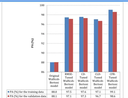
The results for the predicted path loss versus path length for the original Walficsh-Bertoni model and the various tuned Walficsh-Bertoni models are shown in Figure 2 for case where the training dataset is used for the evaluation. Similar results of the predicted path loss versus path length for the original Walficsh-Bertoni model and the various tuned Walficsh-Walficsh-Bertoni models are shown in Figure 3 for case where the validation dataset is used. The prediction performance, RMSE (dB) and MAPE (dB), for the original Walficsh-Bertoni model and the various tuned Walficsh-Bertoni models for case where the training and validation datasets are used is shown in Figure 4 while the prediction accuracy is shown in Figure 5. The results show that the CFR-Tuned Walficsh-Bertoni model has the best prediction performance with the least RMSE of 1.5 dB, least MAPE of 1.2 dB and the highest prediction accuracy, PA of 99.1%. It also maintained the best prediction performance with the validation dataset. The CD-tuned Walficsh-Bertoni model is the second, followed by the popular RMSE-tuned Walficsh-Bertoni model. Among the four tuning methods considered, the CLD-tuned Walficsh-Bertoni model had the least prediction performance.

The tuned models are then derived based on the tuned parameters. Now, the RMSE = 16.1 dB, then , the RMSE-based tuning model becomes;

𝑃_{𝑊𝐵_𝑅𝑀𝑆𝐸(𝑖)}= 89.5 − 10 (log₁₀( 𝜌1𝑅0.9

(𝐻𝐵−ℎ𝑚)2)) +

21(log₁₀(𝑓_𝑚)) − 18(log₁₀(ℎ_𝑏− 𝐻_𝐵)) + 38(log10(𝑑)) +16.1 (10) When the constants are added, the RMSE-tuned

model becomes; 𝑃𝑊𝐵_𝑅𝑀𝑆𝐸(𝑖)= 105.6 − 10 (log10(

𝜌1𝑅0.9

(𝐻𝐵−ℎ𝑚)2)) +

21(log10(𝑓𝑚)) − 18(log10(ℎ𝑏− 𝐻𝐵)) + 38(log10(𝑑)) (11) In the case of the CD-tuning method, the parameter, 𝐾_𝐶𝐷 = 2.58 , then,

𝑃𝑊𝐵_𝐶𝐷(𝑖) = 89.5 − 10 (log10( 𝜌1𝑅0.9

(𝐻𝐵−ℎ𝑚)2)) +

21(log10(𝑓𝑚)) − 18(log10(ℎ𝑏− 𝐻𝐵)) + 38(log₁₀(2.58𝑑)) (12) In the case of the CLD-tuning method, the parameter, 𝐾_𝐶𝐿𝐷= 0.1 , hence,

𝑃𝑊𝐵_𝐶𝐿𝐷(𝑖)= 89.5 − 10 (log10( 𝜌1𝑅0.9

(𝐻𝐵−ℎ𝑚)2)) +

21(log10(𝑓𝑚)) − 18(log10(ℎ𝑏− 𝐻𝐵)) + 3.8(log10(𝑑)) (13) Finally, the composition function of residue, 𝑓(𝑒 𝑜𝑓 𝑑) is given as;

𝑓(𝑒 𝑜𝑓 𝑑) = 161.1(d) -99.56 (14) Hence;

𝑃_{𝑊𝐵_𝐶𝐹𝑅(𝑖)}= 89.5 − 10 (𝑙𝑜𝑔₁₀( 𝜌1𝑅0.9

(𝐻𝐵−ℎ𝑚)2)) +

21(𝑙𝑜𝑔₁₀(𝑓𝑚)) − 18(𝑙𝑜𝑔10(ℎ𝑏− 𝐻𝐵)) + 38(𝑙𝑜𝑔10(𝑑))+161.1(d) -99.56 (15)

In all, while the RMSE is the most popular method used for tuning path loss models, the results have shown that there are also simple methods that can give better prediction accuracy than the RMSE method.

Figure 2 The predicted path loss versus path length for the original Walficsh-Bertoni model and the various tuned Walficsh-Bertoni models for case where the training dataset is used

110 115 120 125 130 135 140

0.65 0.7 0.75 0.8

P

ath

Loss

(dB)

Path Length, d (Km)

Field Measured Path Loss (dB) Original Walficsh-Bertoni model RMSE-Tuned Walficsh-Bertoni model

CD-Tuned Walficsh-Bertoni model CLD-Tuned Walficsh-Bertoni model

(4)

Vol. 4 Issue 12, December - 2018

Figure 3 The predicted path loss versus path length for the original Walficsh-Bertoni model and the various tuned Walficsh-Bertoni models for case where the validation dataset is used

Figure 4 The prediction performance, RMSE (dB) and MAPE (dB), for the original Walficsh-Bertoni model and the various tuned Walficsh-Bertoni models for case where the training and validation datasets are used

112 117 122 127 132 137 142

0.67 0.72 0.77

P

ath

Loss

(dB)

Path Length (Km)

Field Measured Path Loss (dB) Original Walficsh-Bertoni model RMSE-Tuned Walficsh-Bertoni model

CD-Tuned Walficsh-Bertoni model

CLD-Tuned Walficsh-Bertoni model

CFR-Tuned Walficsh-Bertoni model

Original

Walficsh-Bertoni model

RMSE-Tuned

CD-Tuned

CLD-Tuned

CFR-Tuned

RMSE (dB) for the training data 16.1 3.8 3.8 4.4 1.5

RMSE (dB) for the validation

data 16.2 4.4 4.4 4.9 2.2

MAPE (dB) for the training data 15.7 3.3 3.2 3.8 1.2

MAPE (dB) for the validation

data 15.7 3.7 3.5 4.3 1.8

0.2 1.2 2.2 3.2 4.2 5.2 6.2 7.2 8.2 9.2 10.2 11.2 12.2 13.2 14.2 15.2 16.2

R

MSE (dB)

and

MAP

E (dB

(5)

Figure 5 The percentage accuracy, PA(%), for the original Bertoni model and the various tuned Walficsh-Bertoni models for case where the training and validation datasets are used

VI. CONCLUSION

Four different methods for optimizing the Walficsh-Bertoni path loss model are presented and their path loss prediction performances are compared. The prediction performance is based on empirical path loss data collected through field measurement conducted in a timber market located on the outskirts of Uyo in Akwa Ibom State. Specifically, the 3G cellular network was considered in the study and the received signal strength intensity (RSSI), the transmitting base station information and other relevant information required for the study were collected with the use of G-NetTrack Lite 8.0 wireless network site surveying android app installed on Samsung Galaxy S8 phone. The results showed that among the four different model optimization methods considered, the composition function of residue tuning method gave the best prediction performance. The popularly used root mean square error (RMSE) method was third in the prediction performance ranking. In all, this paper has demonstrated that while the RMSE method is popular, there are other simple tuning methods that can perform better.

REFERENCES

1. Chebil, J., Lawas, A. K., & Islam, M. D. (2013). Comparison between measured and predicted path loss for mobile communication in Malaysia. World Applied Sciences Journal, 21, 123-128.

2. ABA, R. O. (2014). PATH LOSS PREDICTION FOR GSM MOBILE NETWORKS FOR URBAN REGION OF ABA, SOUTH-EAST NIGERIA. 3. Plets, D., Joseph, W., Vanhecke, K., Tanghe, E., &

Martens, L. (2013). Simple indoor path loss prediction algorithm and validation in living lab setting. Wireless Personal Communications, 68(3), 535-552.

4. Plets, D., Mangelschots, R., Vanhecke, K., Martens, L., & Joseph, W. (2016). A mobile app for real-time testing of path-loss models and

optimization of network planning. In 27th IEEE Annual International Symposium on Personal, Indoor, and Mobile Radio Communications (PIMRC) (pp. 2507-2513).

5. Hoomod, H. K., Al-Mejibli, I., & Jabboory, A. I. (2018, May). Analyzing Study of Path loss Propagation Models in Wireless Communications at 0.8 GHz. In Journal of Physics: Conference Series (Vol. 1003, No. 1, p. 012028). IOP Publishing.

6. Popoola, S. I., Adetiba, E., Atayero, A. A., Faruk, N., & Calafate, C. T. (2018). Optimal model for path loss predictions using feed-forward neural networks. Cogent Engineering, 5(1), 1444345. 7. Han, S. Y., Abu-Ghazaleh, N. B., & Lee, D. (2016).

Efficient and consistent path loss model for mobile network simulation. IEEE/ACM Transactions on Networking (TON), 24(3), 1774-1786.

8. Bola, G. S., & Saini, G. S. (2013). Path Loss Measurement and Estimation Using Different Empirical Models For WiMax In Urban Area.

Original

RMSE-Tuned

CD-Tuned

CLD-Tuned

CFR-Tuned

PA (%) for the training data 88.0 97.5 97.6 97.1 99.1

PA (%) for the validation data 88.1 97.1 97.3 96.7 98.6

86 88 90 92 94 96 98 100

P

A

(6)

Vol. 4 Issue 12, December - 2018

International Journal of Scientific & Engineering Research, 4(5), 1421-1428.

9. Segun, A., Akinwunmi, A. O., & Ogunti, E. O. (2015). A survey of medium access control protocols in wireless sensor network. International Journal of Computer Applications, 116(22). 10. Nurminen, H., Talvitie, J., Ali-Löytty, S., Müller, P.,

Lohan, E. S., Piché, R., & Renfors, M. (2013). Statistical path loss parameter estimation and positioning using RSS measurements. Journal of Global Positioning Systems, 12(1), 13-27. 11. Hu, Y., & Leus, G. (2015). Self-estimation of

path-loss exponent in wireless networks and applications. IEEE Transactions on Vehicular Technology, 64(11), 5091-5102.

12. Hoomod, H. K., Al-Mejibli, I., & Jabboory, A. I. (2018, May). Analyzing Study of Path loss Propagation Models in Wireless Communications at 0.8 GHz. In Journal of Physics: Conference Series (Vol. 1003, No. 1, p. 012028). IOP Publishing.

13. Gustafson, C., Abbas, T., Bolin, D., & Tufvesson, F. (2015). Statistical modeling and estimation of censored pathloss data. IEEE Wireless

Communications Letters, 4(5), 569-572. 14. Akinwole, B. O. H., & Biebuma, J. J. (2013).

Comparative Analysis Of Empirical Path Loss Model For Cellular Transmission In Rivers State.

Jurnal Ilmiah Electrical/Electronic Engineering, 2, 24-31.

15. Adeyemi, A., Oluwadamilola, A., Aderemi, A., & Francis, I. (2014). A Performance Review of the Different Path Loss Models for LTE Network Planning. In Proceedings of the World Congress on Engineering (Vol. 1).

16. Singh, Y. (2012). Comparison of okumura, hata and cost-231 models on the basis of path loss and signal strength. International journal of computer applications, 59(11).

17. Roslee, M. B., & Kwan, K. F. (2010). Optimization of Hata propagation prediction model in suburban area in Malaysia. Progress in electromagnetics research, 13, 91-106.

18. Akinwole, B. O. H., & Biebuma, J. J. (2013). Comparative Analysis Of Empirical Path Loss Model For Cellular Transmission In Rivers State.

Jurnal Ilmiah Electrical/Electronic Engineering, 2, 24-31.

19. Ranvier, S. (2004). Path loss models. Helsinki University of Technology.

20. Chrysikos, T., Georgopoulos, G., & Kotsopoulos, S. (2009, June). Site-specific validation of ITU indoor path loss model at 2.4 GHz. In World of Wireless, Mobile and Multimedia Networks & Workshops, 2009. WoWMoM 2009. IEEE International Symposium on A (pp. 1-6). IEEE. 21. Nurminen, H., Talvitie, J., Ali-Löytty, S., Müller, P.,

Lohan, E. S., Piché, R., & Renfors, M. (2013). Statistical path loss parameter estimation and positioning using RSS measurements. Journal of Global Positioning Systems, 12(1), 13-27.

22. Zegarra, J. (2015). Model development for wireless propagation in forested environments. Naval Postgraduate School Monterey United States. 23. Faruk, N., Ayeni, A., & Adediran, Y. A. (2013). On

the study of empirical path loss models for accurate prediction of TV signal for secondary

24. Alam, D., & Khan, R. H. (2013). Comparative study of path loss models of WiMAX at 2.5 GHz

frequency band. International Journal of Future Generation Communication and Networking, 6(2), 11-24.

25. Sun, S., Rappaport, T. S., Rangan, S., Thomas, T. A., Ghosh, A., Kovacs, I. Z., ... & Jarvelainen, J. (2016, May). Propagation path loss models for 5G urban micro-and macro-cellular scenarios. In

Vehicular Technology Conference (VTC Spring), 2016 IEEE 83rd (pp. 1-6). IEEE

26. Piersanti, S., Annoni, L. A., & Cassioli, D. (2012, June). Millimeter waves channel measurements and path loss models. In Communications (ICC), 2012 IEEE International Conference on (pp. 4552-4556). IEEE.

27. Liechty, L. C. (2007). Path loss measurements and model analysis of a 2.4 GHz wireless network in an outdoor environment (Doctoral dissertation, Georgia Institute of Technology).

28. Karedal, J., Czink, N., Paier, A., Tufvesson, F., & Molisch, A. F. (2011). Path loss modeling for vehicle-to-vehicle communications. IEEE transactions on vehicular technology, 60(1), 323-328.

29. Phillips, C., Sicker, D., & Grunwald, D. (2011, May). Bounding the error of path loss models. In

New Frontiers in Dynamic Spectrum Access Networks (DySPAN), 2011 IEEE Symposium on

(pp. 71-82). IEEE.

30. Joshi, S., & Gupta, V. (2012). A Review on Empirical data collection and analysis of Bertoni's model at 1. 8 GHz. International Journal of Computer Applications, 56(6).

31. Hernández-Pérez, E., Navarro-Mesa, J. L., Martin-Gonzalez, S., Quintana-Morales, P., & Ravelo-Garcia, A. (2011, August). Path loss factor estimation for RSS-based localization algorithms with wireless sensor networks. In Signal

Processing Conference, 2011 19th European (pp. 1994-1998). IEEE.

32. Nagy, L., & Nagy, B. (1994, September).

Comparison and verification of urban propagation models. In 5th IEEE International Symposium on Personal, Indoor and Mobile Radio

Communications (Vol. 4, pp. 1359-1363). 33. Singh, Y. (2012). Comparison of okumura, hata

and cost-231 models on the basis of path loss and signal strength. International journal of computer applications, 59(11).