www.the-cryosphere.net/2/95/2008/
© Author(s) 2008. This work is distributed under the Creative Commons Attribution 3.0 License.
The Cryosphere
Benchmark experiments for higher-order and full-Stokes ice sheet
models (ISMIP–HOM)
∗
F. Pattyn1, L. Perichon1, A. Aschwanden2, B. Breuer3, B. de Smedt4, O. Gagliardini5, G. H. Gudmundsson6, R. C. A. Hindmarsh6, A. Hubbard7, J. V. Johnson8, T. Kleiner3, Y. Konovalov9, C. Martin6, A. J. Payne10, D. Pollard11, S. Price10, M. R ¨uckamp3, F. Saito12, O. Souˇcek13, S. Sugiyama14, and T. Zwinger15
1Laboratoire de Glaciologie, Universit´e Libre de Bruxelles, CP160/03, Av. F. Roosevelt 50, 1050 Brussels, Belgium 2Institute for Atmospheric and Climate Science, ETH Zurich, Universitaetstrasse 16, 8092 Zurich, Switzerland 3Institute for Geophysics, University of Muenster, Corrensstrasse 24, 48149 Muenster, Germany
4Vakgroep Geografie, Vrije Universiteit Brussel, Pleinlaan 2, 1050 Brussels, Belgium
5Laboratoire de Glaciologie et de G´eophysique de l’Environnement (LGGE), CNRS, UJF-Grenoble I, BP 96, 38402 Saint
Martin d’H`eres Cedex, France
6Physical Science Division, British Antarctic Survey, Natural Environment Research Council, High Cross, Madingley Road,
Cambridge CB3 0ET, UK
7Centre for Glaciology, Institute of Geography and Earth Sciences, Aberystwyth University, Ceredigion, SY23 3DP, UK 8Department of Computer Science, Social Science Building Room 417, Univ. of Montana, Missoula MT, 59812-5256, USA 9Moscow Engineering Physics Institute, Moscow, Russia
10Bristol Glaciology Centre, School of Geographical Sciences, University Road, University of Bristol, Bristol BS8 1SS, UK 11Earth and Environmental Systems Institute, College of Earth and Mineral Sciences, 2217 Earth-Engineering Sciences Bldg.,
Pennsylvania State University, University Park, PA 16802, USA
12Frontier Res. Center for Global Change, 3173-25 Showamachi, Kanazawa-ku, Yokohama City, Kanagawa 236-0001, Japan 13Department of Geophysics, Charles University Prague, V. Holeˇsoviˇck´ach 2, 18000 Praha 8, Czech Republic
14Institute of Low Temperature Science, Hokkaido University, Nishi-8, Kita-19, Sapporo 060-0819, Japan 15CSC-Scientific Computing Ltd., Keilaranta 14, P.O. Box 405, 02101 Espoo, Finland
∗Ice Sheet Model Intercomparison Project for Higher-Order Models; http://homepages.ulb.ac.be/∼fpattyn/ismip Received: 20 December 2007 – Published in The Cryosphere Discuss.: 19 February 2008
Revised: 7 July 2008 – Accepted: 8 August 2008 – Published: 26 August 2008
Abstract. We present the results of the first ice sheet model intercomparison project for higher-order and full-Stokes ice sheet models. These models are compared and verified in a series of six experiments of which one has an analytical solution obtained from a perturbation analysis. The experi-ments are applied to both 2-D and 3-D geometries; five ex-periments are steady-state diagnostic, and one has a time-dependent prognostic solution. All participating models give results that are in close agreement. A clear distinction can be made between higher-order models and those that solve the full system of equations. The full-Stokes models show a much smaller spread, hence are in better agreement with one another and with the analytical solution.
Correspondence to: F. Pattyn
1 Introduction
Despite the lack of comprehensive predictive ice sheet modeling, the ice sheet modeling community has evolved considerably over the last decade. Increasing computational power has led to the development of more complex ice sheet models, with varying degrees of approximations to the Stokes equations. However, progress has been hampered by the lack of a universal verification framework and in particu-lar by a lack of full-Stokes analytical solutions. While meth-ods exist for constructing exact solutions to the Newtonian full-Stokes equations in the flowline case (e.g. Ladyzhen-skaya, 1969), obtaining analytical solutions for the 3-D case is less straightforward. Nevertheless, solutions based on per-turbation analysis exist (e.g. Gudmundsson, 2003), and were used for this study. Benchmark validation exercises were car-ried out on large-scale ice-sheet and ice-shelf models in the 1990s (Huybrechts et al., 1996; MacAyeal et al., 1996; Payne et al., 2000), but these tests were largely restricted to zero-order (SIA) models and solutions. Here we present an in-tercomparison exercise which involves 28 higher-order flow models of varying complexity. The experiments described in this paper are designed to evaluate the conditions under which different higher-order solutions are viable and to de-termine whether numerical issues affect the result.
During the first and second EISMINT1model intercom-parison exercises, a number of benchmarks were proposed specifically for ice sheet models (Huybrechts et al., 1996, 1998; Payne et al., 2000) and ice shelf models (MacAyeal et al., 1996). These ice sheet models were based on the zeroth-order shallow-ice approximation (SIA; Hutter, 1983), incorporating only vertical shear stresses in the force bal-ance. The ISMIP-HOM exercise focuses on so-called higher-order models, i.e. models that incorporate further mechanical effects, principally longitudinal stress gradients, as well as those that solve the full system of equations of the Stokes problem.
The six experiments which comprise this benchmark exer-cise are designed to be universally accessible to many differ-ent types of models, i.e. flowline (2-D), vertically integrated planform (2.5-D) and full 3-D models. Furthermore, the ex-periments are defined as well-posed continuum problems so that their application is not limited to any specific numeri-cal methodology. The equations have been solved using well established finite-difference and finite-element methods, in addition to more esoteric spectral techniques. The latter hold particular promise for providing high-quality results in the absence of analytical solutions, but since only one partici-pant provided spectral model results, they were not isolated for comparison.
With the exception of Exp. F, all experiments are diag-nostic; i.e. time evolution is not considered. This means that for a given ice geometry, a Glen-type flow law, and ap-propriate boundary conditions, the stress and velocity fields
1EISMINT: European Ice Sheet Model INTercomparison; http:
//homepages.vub.ac.be/∼phuybrec/eismint.html
can be calculated. Exp. F considers the time-dependent re-sponse (the experiment is run until the free surface and ve-locity field reach a steady state) for a constant viscosity (lin-ear flow law). Constant viscosity is assumed because in this case there exist analytic solutions derived from a first-order perturbation analysis of flow down an inclined plane (Gud-mundsson, 2003). In all experiments, thermomechanical ef-fects are neglected and ice is considered to be isothermal and isotropic.
2 General model setup
2.1 Model physics, parameters and constants
Higher-order models are ice-sheet or glacier models that in-corporate effects not present in the shallow-ice approxima-tion. In most cases this implies the inclusion of longitudi-nal stress gradients apart from the two horizontal-plane shear components (Hindmarsh, 2004). Longitudinal stresses have recently been termed “membrane stresses” when considered in three dimensions (Hindmarsh, 2006). The suite of models is based on conservation laws of mass and momentum, i.e.
∇ ·v=0, (1)
ρdv
dt = ∇ ·T+ρg, (2)
whereρ is the ice density, g is gravitational acceleration, v is the velocity vector, and T is the stress tensor. Values for parameters and constants are given in Table 1. Generally, acceleration terms in Eq. (2) are neglected. Ice incompress-ibility is more easily described if the stress tensor is split into a deviatoric part and an isotropic pressureP,
T=T0−PI, (3)
whereP=−1
3tr(T). The constitutive equation for ice then
links deviatoric stresses to strain rates:
T0=2ηe˙, (4)
where T0ande are the deviatoric stress and strain-rate tensor,˙ respectively, andηis the effective viscosity. Both linear and nonlinear ice rheologies are considered. In the latter case (Glen’s flow law),ηis strain-rate dependent and defined by
η= 1
2A
−1/nε˙(1−n)/n
e , (5)
whereε˙e is the effective strain rate. For the case of linear
rheology, Eq. (5) reduces toη=(2A)−1, whereAis spatially uniform (i.e., the ice is isothermal). Neglecting acceleration terms, the momentum balance is written as:
Table 1. Constants for the numerical model.
Constant Value Units
A Ice-flow parameter 10−16 Pa−na−1
ρ Ice density 910 kg m−3
g Gravitational constant 9.81 m s−2
n Exponent in Glen’s flow law 3
Seconds per year 31 556 926 s a−1
Since acceleration due to gravity acts only in the vertical, this leads to
∂τxx0
∂x −
∂P
∂x +
∂τxy0
∂y +
∂τxz0
∂z =0, (7)
∂τyx0
∂x +
∂τyy0
∂y −
∂P
∂y +
∂τyz0
∂z =0, (8)
∂τzx0
∂x +
∂τzy0
∂y +
∂τzz0
∂z −
∂P
∂z =ρg . (9)
Solving Eqs. (7)–(9) leads to the full-Stokes solution. Sim-plifications of these equations lead to the various higher-order approximations discussed below.
2.2 Boundary conditions
In Exps. A, B, E1 and F1 the ice is frozen to the bed (vb=0). For the other experiments, basal sliding is introduced through a friction law, characterized by a friction coefficientβ2. This friction law has the form of
β2t·v=t·(Tnb)=τb, (10)
where nbis the unit normal vector pointing into the bedrock,
t is the unit tangent vector, and β2 (Pa a m−1) is a posi-tive scalar (MacAyeal, 1993). Basal shear stress τb is not
equal to the driving stress but is part of the solution. The stress is negligible at the upper ice surface, implying that ns·(Tns)=Patm≈0.
Kinematic boundary conditions apply at the upper and lower surfaces of the ice mass, i.e.
∂zi
∂t +vx(zi) ∂zi
∂x +vy(zi) ∂zi
∂y −vz(zi)=0, (11)
fori=(s, b). Since the vertical velocity field must obey the incompressibility condition Eq. (1), and the surface accumu-lation/ablation is zero, the vertical velocity at the surface con-tains the local imbalance as well and becomes a model out-put.
2.3 Model domain
For the 3-D experiments the model domain is a square of side L, and for 2-D experiments the domain is a flowline of length
Lin thex−zplane. The minimum number of grid points is
−2500 −2200 −2200 −2000 −2000 −1800 −1800 −1800 −1600 −1600 −1600 −1400 −1400 −1200 −1200 −900
Horizontal scaled distance x
Horizontal scaled distance y
0 0.25 0.5 0.75 1
0 0.25 0.5 0.75 1
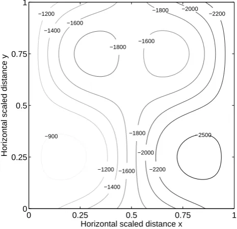
Fig. 1. Basal topographyzb(m) for Exp. A according to Eq. (13)
forL=80 km. Ice flow is from left to right.
not predefined, and any type of discretization scheme can be used. The number of grid points in the horizontal and vertical directions can be chosen freely. The basic parameter for the experiments is the length scaleLof the domain. Exps. A–D are carried out forL=160, 80, 40, 20, 10 and 5 km, respec-tively, which results in aspect ratios =H /L varying from 0.006 to 0.2. Periodic boundary conditions are applied in the horizontal, so that the domain is surrounded by an infinite number of copies of itself.
3 Experiment description
3.1 Exp. A: Ice flow over a bumpy bed
Exp. A considers a parallel-sided slab of ice with a mean ice thicknessH=1000 m lying on a sloping bed with a mean slopeα=0.5◦. This slope is maximum inxand zero iny. The basal topography is then defined as a series of sinusoidal os-cillations with an amplitude of 500 m. The surface elevation is defined as
zs(x, y)= −x·tanα . (12)
The basal topography is then given by
zb(x, y)=zs(x, y)−1000+500 sin(ω x)·sin(ω y) ,(13)
50
50 250
250 650
650 900
900
1150
1150
1500
1500
1850
1850
Horizontal scaled distance x
Horizontal scaled distance y
0 0.25 0.5 0.75 1
0 0.25 0.5 0.75 1
Fig. 2. Basal friction coefficientβ2for Exp. C.
3.2 Exp. B: Ice flow over a rippled bed
The only difference with Exp. A is that the basal topography does not vary withy, so that the experiment is suitable for 2-D flowline models as well. The basal topography is thus formed by a series of ripples with an amplitude of 500 m:
zs(x, y)= −x·tanα (14)
zb(x, y)=zs(x, y)−1000+500 sin(ω x) . (15)
3.3 Exp. C: Ice stream flow I
The experiment setup is similar to Exp. A, except that the bedrock topography is flat, so that the ice thickness is spa-tially uniform (H=1000 m):
zs(x, y)= −x·tanα (16)
zb(x, y)=zs(x, y)−1000, (17)
wherex ∈ [0, L]andL=160, 80, 40, 20, 10 and 5 km, re-spectively, and whereα=0.1◦. The basal friction coefficient is prescribed as
β2(x, y)=1000+1000 sin(ω x)·sin(ω y) . (18)
Theβ2-field is shown in Fig. 2. The basal friction oscilla-tions have a frequencyω=2π/L.
3.4 Exp. D: Ice stream flow II
The only difference with Exp. C is that the basal friction co-efficient does not vary withy, so that the experiment is suited
0 1 2 3 4 5
2500 2600 2700 2800 2900 3000 3100 3200
Elevation (m)
Distance (km)
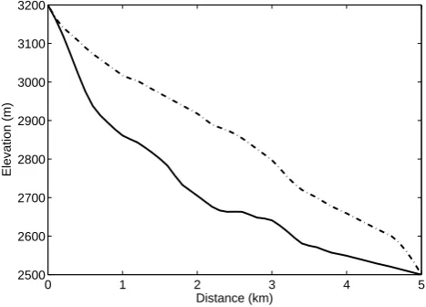
Fig. 3. Surface and bedrock profile of Haut Glacier d’Arolla.
for 2-D flowline models as well. The basal friction field is thus formed by a series of ripples defined as
β2(x, y)=1000+1000 sin(ω x) . (19)
Note that in Exps. C and D the basal friction coefficientβ2
goes to zero within the domain.
3.5 Exp. E: Haut Glacier d’Arolla
Exp. E is a diagnostic experiment along the central flow-line of a temperate glacier in the European Alps (Haut Glacier d’Arolla), based on earlier experiments by Blatter et al. (1998) and Pattyn (2002). Model input consists of the longitudinal surface and bedrock profiles of Haut Glacier d’Arolla, Switzerland, according to the Little Ice Age ge-ometry (Fig. 3). The longitudinal profile of this glacier has a very simple geometry, hence the resulting stress field is not influenced by geometrical perturbations such as the pres-ence of a steep ice fall. In a first experiment (E1), a zero basal velocity is considered (β2=∞), and the width of the drainage basin is kept equal to 1 along the entire flowline. The flow-law rate factorA=10−16Pa−na−1is assumed con-stant. Upstream and downstream boundary conditions imply zero ice thickness and velocity. The input file has a resolu-tion1x=100 m, but the authors were free to choose any grid resolution.
A second experiment (E2) considers a narrow zone of zero traction, similar to the experiment described in Blatter et al. (1998):
3.6 Exp. F: Prognostic experiment
Exp. F is a prognostic experiment for which the free surface is allowed to relax until a steady state is reached for zero surface mass balance:
lim
t→∞
∂H
∂t =tlim→∞
−∇h·
zs
Z
zb vhdz
=0, (20)
where vh is the horizontal velocity vector (m a−1). Basic
model setup differs from the setup in Exps. A and C. A slab of ice with mean ice thicknessH(0)=1000 m is considered, resting on a sloping bed with a mean slopeα=3.0◦(Fig. 4). This slope is maximum inxand zero iny. The bedrock plane is parallel to the surface plane and is perturbed by a Gaussian bump. Initial bedrockB(0)and unperturbed surfaceS(0) ele-vation are thus governed by
S(0)(x, y)=0 (21)
B(0)(x, y)= −H(0)+a0 exp "
−(x2+y2) σ2
#!
, (22)
whereσ=10000m=10H(0)and wherex, y (m) are the hor-izontal coordinates with respect to the center of the Gaus-sian bump. The basal perturbation has a maximum height of one-tenth of the mean ice thickness, i.e.a0=100=0.1H(0)
(Fig. 4). The domain sizeLis taken to be 100H(0)inx and
y. The horizontal coordinates for output are scaled by ˆ
x= x
H(0) yˆ =
y
H(0) . (23)
Periodic boundary conditions are applied in the horizontal. The major difference with the previous experiments is that
n=1 in Eq. (5), so that the effective viscosity is constant and becomesη=(2A)−1. Therefore, the unperturbed veloc-ity field at the surface is defined by
U(0)=AH(0)τb(0) =ρgAhH(0)i2sinα , (24) where τb(0)=ρgH(0)sinα is the unperturbed basal shear stress, and A=2.140373×10⁻⁷Pa−1a−1, so that
U(0)=100 m a−1.
Experiments are carried out for different values of the slip ratioc, which determines the relation between the basal ve-locity and basal drag. The basal veve-locity is written in terms of a basal friction coefficientβ2, or
Ub=
τb
β2 . (25)
Following the scalings given by Gudmundsson (2003), the basal friction coefficient is related to the slip ratiocby
β2=cAH(0)
−1
. (26)
0
−900
−1000
α
Fig. 4. Tilted coordinate system used for Exp. F.
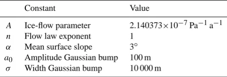
Table 2. Constants for the model setup according to Exp. F.
Constant Value
A Ice-flow parameter 2.140373×10⁻⁷Pa−1a−1
n Flow law exponent 1
α Mean surface slope 3◦
a0 Amplitude Gaussian bump 100 m
σ Width Gaussian bump 10 000 m
Experiments are run for slip ratios c=0 and 1 (F1 and F2, respectively). It is easily demonstrated thatUb(0)=cU(0). Ta-ble 2 lists the main constants used for Exp. F. Using these settings, the model should run until a steady state of the free surface is reached.
4 Model classification
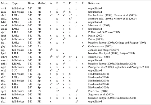
Table 3. List with the 28 participating models. Model: model acronym based on the initials of each author; Type: the model type (see text
for description); Dims: model dimensions; Method: numerical method (FE = finite elements, FD = finite differences, Sp = spectral method, FV = finite volume, An = analytical); A–F participation in the different experiments is marked with an x.
Model Type Dims Method A B C D E F Reference
aas1 full-Stokes 2-D FE x x x unpublished
aas2 full-Stokes 3-D FE x x xa x unpublished
ahu1 LMLa 3-D FD xa xa xa xa x Hubbard et al. (1998); Nienow et al. (2005)
ahu2 LMLa 2-D FD x xc Hubbard et al. (1998); Nienow et al. (2005)
bds1 LMLa 2-D FE x x x unpublished
cma1 full-Stokes 3-D FE x x x x x x Martin et al. (2003)
cma2 LMLa 3-D FE x x x x x unpublished
dpo1 L1L2 2-D FD x x Pollard and DeConto (2007)
fpa1 LMLa 3-D FD x x x x x x Pattyn (2003)
fpa2 full-Stokes 3-D FD xc xb Pattyn (2008)
fsa1 LMLa 3-D FD x x x x based on Pattyn (2003); Colinge and Rappaz (1999)
ghg1 full-Stokes 3-D An xd Gudmundsson (2003)
jvj1 full-Stokes 3-D FE xb x Johnson and Staiger (2007)
lpe1 L1L1 2-D FD x based on MacAyeal (1989); Pattyn (2003)
mbr1 LMLa 3-D FD xb xb xc xc x x Breuer et al. (2006)
mmr1 full-Stokes 3-D FE x x x x unpublished
mtk1 LTSML 3-D FD x x xa x based on Pattyn (2003); Hindmarsh (2004)
oga1 full-Stokes 3-D FE x x x x x x Zwinger et al. (2007); Gagliardini and Zwinger (2008)
oso1 SIA’ 3-D xa xa unpublished
rhi1 full-Stokes 3-D Sp x x x x Hindmarsh (2004)
rhi2 LMLa 3-D Sp x x x x Hindmarsh (2004)
rhi3 full-Stokes 3-D Sp x x x x Hindmarsh (2004)
rhi4 L1L2 3-D Sp xa xa x x Hindmarsh (2004)
rhi5 L1L1 3-D Sp x x x x Hindmarsh (2004)
spr1 full-Stokes 2-D FV xa xd Price et al. (2007)
ssu1 full-Stokes 2-D FE x x x Sugiyama et al. (2003)
tpa1 LMLa 3-D FD x x x x x based on Pattyn (2003); Hindmarsh (2004)
yko1 full-Stokes 3-D FD x xd unpublished
anot forL=5 km bnot forL=5 and 10 km cnot forL=5, 10 and 20 km donly no-sliding case
elevation only (generally the upper surface), giving a com-putationally two-dimensional problem. These higher-order approximations are labeled L1L1, L1L2, LMLa and LTSML (Hindmarsh, 2004).
The L1L1 approximation is a one-layer longitudinal stress scheme usingτxx0 at the surface computed by solving ellip-tic equations and is idenellip-tical to the approximation used by MacAyeal (1989). An alternative approximation is the L1L2 approach, or one-layer longitudinal stress scheme, usingε˙xx
at the surface computed by solving elliptical equations with a vertical correction ofτxx0 . Here, the surface velocities used in computing the non-horizontal plane stresses are computed using the vertical shear stresses in the shear strain relation-ship and in the sliding relationrelation-ship.
The most common approximation is the LMLa or multi-layer longitudinal stress scheme. This is the classic
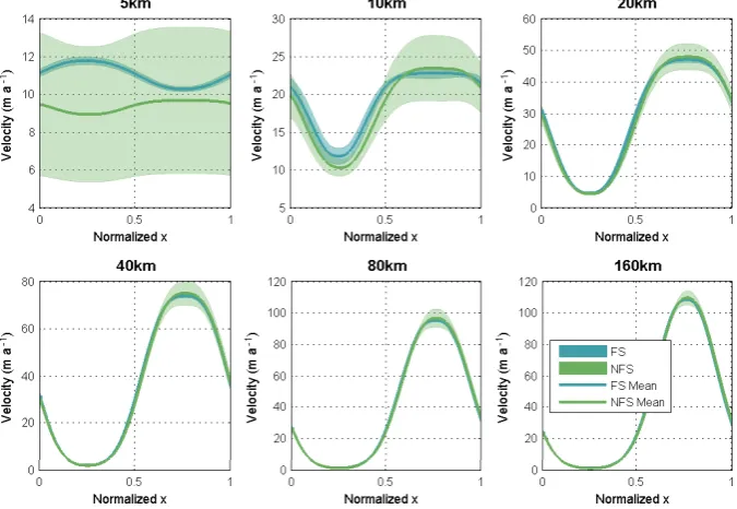
Fig. 5. Results for Exp. A: norm of the surface velocity across the bump aty=L/4 for different length scalesL. The mean value and standard deviation are shown for both types of models.
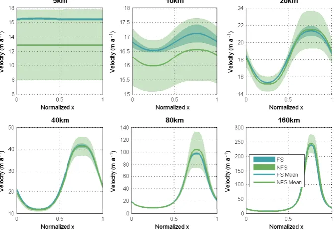
Fig. 6. Results for Exp. B: norm of the surface velocity for different length scalesL. The mean value and standard deviation are shown for both types of models.
5 Results
A graphical representation of all the results for each of the contributing authors as well as the submitted data files are found in the supplemental files http://www.the-cryosphere. net/2/95/2008/tc-2-95-2008-supplement.zip. The detailed
0 0.1 0.2 0.3 0.4 0.5 0.6 0.7 0.8 0.9 1 0 20 40 60 80 100 120 140
119.69 m a−1
Normalized distance
Surface velocity (m a
−1
)
A & B C & D
Fig. 7. Surface velocity profiles alongy=L/4 according to the an-alytical SIA solution for Exps. A–D, based on Eqs. (27) and (28). Results are independent ofL.
The numerical results are displayed in both numerical and graphical format. A distinction is made between full-Stokes (FS) and non-full-Stokes (NFS) models, such as LMLa, LTSML, L1L2 and L1L1. All parameters refer to horizon-tal surface velocities, which are determined as the norm of the horizontal components of the velocity field, defined by ||vs||=
q v2
x+v2y. Velocities are displayed along a section
y=L/4 for Exps. A and C and along a central liney=L/2 for Exp. F. For the 2-D experiments we show results along the flowline. The graphs show the mean velocity and its standard deviation along each section or flowline for both FS and NFS models. The tables present two parameters for each flowline or section: the maximum value of the norm of the surface velocity and the mean value of the velocity. For both param-eters the mean and standard deviations are given for both FS and NFS models.
5.1 Experiments A and B
The results for Exps. A and B are shown in Figs. 5 and 6, respectively, and the numerical results are given in Tables 4 and 5. Each graph displays the norm of the surface veloc-ity across the bumps aty=L/4 (for Exp. A) and along the central flowline (for Exp. B), for the different length scales and model groups (FS and NFS). The experiments were set up such that for this longitudinal profile the SIA gives a solu-tion independent ofL, which is not the case for higher-order models. The surface velocity according to the SIA is given by
vx(zs)=vx(zb)+
2A
n+1(ρgtanα)
nHn+1, (27)
wherevx(zb)=0 is the basal velocity (Fig. 7). The maximum
surface velocity according to the SIA remains constant for all length scales (119.69 m a−1). However, whenever topo-graphic differences occur, longitudinal stress gradients must
develop which tend to smooth out the velocity field. For high aspect ratios=H /L(hence low values ofL) this leads to a more or less constant surface velocity field as the ice sheet does not “feel” the individual bedrock undulations. Rather, it feels the fast sequence of large bed undulations as a vis-cous drag. The aspect ratio determines the amplitude of the horizontal surface velocity field, and the surface velocity decreases from∼100 to∼10 m a−1.
Full-Stokes models closely agree with each other when calculating the velocity field for different length scales, com-pared to the larger spread of solutions for the higher-order approximations (Tables 4 and 5). Several factors could be responsible for the larger spread among NFS models: (i) More models are participating; (ii) These models are solving different continuum equations (LMLa, LTSML, L1L1, and L1L2); (iii) At the highest aspect ratios, the different approx-imations are not valid, so that the full-stress model needs to be solved; and (iv) There are numerical errors relative to the unknown exact solutions of the continuum equations. The FS results are only subject to a spread from the latter cause. For the smallest length scales the standard deviation for the full-Stokes models reduces to<0.2 m a−1(Tables 4 and 5). The coarsest grid used by the participating models had di-mensions 40×40, leading to a numerical mismatch of the or-der of 2.5%, which is far smaller than the standard deviation shown in Fig. 5 for the higher-order models. It is therefore very likely that the large spread associated with the higher-order models is due to the invalidity of the approximations compared to the full-Stokes solution.
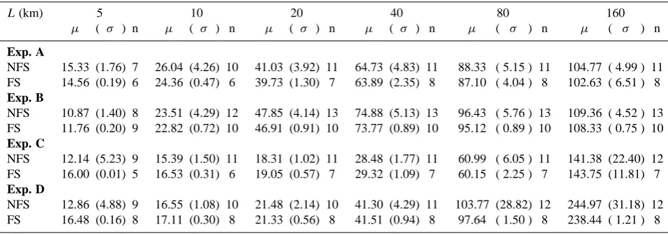
Table 4. Mean values (µ), standard deviation (σ) and number of participating models (n) of the maximum horizontal ice velocity at the surface in the direction of the flow. Results are listed for Exp. A–D and for each length scale. Units are m a−1.
L(km) 5 10 20 40 80 160
µ ( σ ) n µ ( σ ) n µ ( σ ) n µ ( σ ) n µ ( σ ) n µ ( σ ) n
Exp. A
NFS 15.33 (1.76) 7 26.04 (4.26) 10 41.03 (3.92) 11 64.73 (4.83) 11 88.33 ( 5.15 ) 11 104.77 ( 4.99 ) 11 FS 14.56 (0.19) 6 24.36 (0.47) 6 39.73 (1.30) 7 63.89 (2.35) 8 87.10 ( 4.04 ) 8 102.63 ( 6.51 ) 8
Exp. B
NFS 10.87 (1.40) 8 23.51 (4.29) 12 47.85 (4.14) 13 74.88 (5.13) 13 96.43 ( 5.76 ) 13 109.36 ( 4.52 ) 13 FS 11.76 (0.20) 9 22.82 (0.72) 10 46.91 (0.91) 10 73.77 (0.89) 10 95.12 ( 0.89 ) 10 108.33 ( 0.75 ) 10
Exp. C
NFS 12.14 (5.23) 9 15.39 (1.50) 11 18.31 (1.02) 11 28.48 (1.77) 11 60.99 ( 6.05 ) 11 141.38 (22.40) 12 FS 16.00 (0.01) 5 16.53 (0.31) 6 19.05 (0.57) 7 29.32 (1.09) 7 60.15 ( 2.25 ) 7 143.75 (11.81) 7
Exp. D
NFS 12.86 (4.88) 9 16.55 (1.08) 10 21.48 (2.14) 10 41.30 (4.29) 11 103.77 (28.82) 12 244.97 (31.18) 12 FS 16.48 (0.16) 8 17.11 (0.30) 8 21.33 (0.56) 8 41.51 (0.94) 8 97.64 ( 1.50 ) 8 238.44 ( 1.21 ) 8
Table 5. Mean values (µ), standard deviation (σ) and number of participating models (n) of the mean horizontal ice velocity at the surface in the direction of the flow. Results are listed for Exp. A–D and for each length scale. Units are m a−1.
L(km) 5 10 20 40 80 160
µ ( σ ) n µ ( σ ) n µ ( σ ) n µ ( σ ) n µ ( σ ) n µ ( σ ) n
Exp. A
NFS 14.61 (1.79) 7 20.62 (3.23) 10 24.93 (2.20) 11 31.99 (2.07) 11 37.54 (1.58) 11 40.36 (1.07) 11 FS 14.20 (0.18) 6 20.02 (0.36) 6 24.74 (0.79) 7 31.89 (1.07) 8 37.31 (1.30) 8 39.98 (1.52) 8
Exp. B
NFS 10.54 (1.36) 8 18.24 (2.67) 12 27.80 (2.08) 13 35.55 (1.86) 13 39.76 (1.38) 13 41.38 (0.76) 13 FS 11.04 (0.17) 9 19.09 (0.56) 10 28.28 (0.60) 10 35.75 (0.48) 10 39.76 (0.28) 10 41.40 (0.24) 10
Exp. C
NFS 12.12 (5.22) 9 15.19 (1.46) 11 16.36 (0.94) 11 19.25 (0.95) 11 27.24 (1.44) 11 40.83 (3.79) 12 FS 15.99 (0.00) 5 16.24 (0.16) 6 16.84 (0.24) 7 19.76 (0.38) 7 27.38 (0.55) 7 41.68 (1.83) 7
Exp. D
NFS 12.85 (4.88) 9 16.28 (0.97) 10 18.33 (1.13) 10 24.20 (1.09) 11 38.46 (6.48) 12 58.30 (4.86) 12 FS 16.43 (0.16) 8 16.81 (0.18) 8 18.40 (0.24) 8 24.63 (0.29) 8 37.00 (0.33) 8 57.17 (0.35) 8
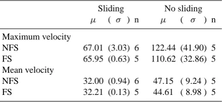
5.2 Experiments C and D
In this series of experiments, variations in basal conditions (slipperiness) determine where longitudinal stress gradients must develop. Due to the importance of basal sliding, the ice behaves as in an ice stream, in which vertical shearing is present, though minimal. Ice flow in this experiment can be considered as ice shelf flow with minimal basal traction. The invalidity of the SIA solution is shown in Fig. 7, where the analytical SIA solution is plotted for a simplified basal slid-ing relationship in which the basal shear stress is supposed to balance the driving stress without longitudinal stress gra-dients, so that
vx(zb)=(ρgHtanα) β−2, (28)
approxima-Table 6. Mean values (µ), standard deviation (σ) and number of participating models (n) of the maximum and mean horizontal ice velocity at the surface in the direction of the flow for Exp. E. Units are m a−1.
Sliding No sliding
µ ( σ ) n µ ( σ ) n
Maximum velocity
NFS 67.01 (3.03) 6 122.44 (41.90) 5
FS 65.95 (0.63) 5 110.62 (32.86) 5
Mean velocity
NFS 32.00 (0.94) 6 47.15 ( 9.24 ) 5
FS 32.21 (0.13) 5 44.61 ( 8.98 ) 5
tions this is not observed (but due to the larger disparity in solutions, this effect is unnoticeable in Fig. 9).
In general, the spread in results of the modeled velocity field is higher than for the experiments over the bedrock bumps. The smallest spread is obtained with full-Stokes models, and this spread reduces with increasing, contrary to the results from Exps. A–B. L1L1 and L1L2 models have larger spreads than the LMLa models, despite the fact that they were designed for coping with such type of ice flow in the first place.
5.3 Experiment E: Haut Glacier d’Arolla
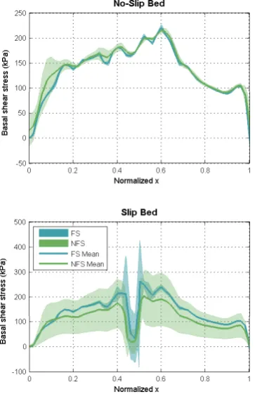
Although the input file lists the bedrock and surface data along the flowline of Haut Glacier d’Arolla with a fixed grid spacing of 1x=100 m, most participants interpolated this dataset at a higher resolution (Fig. 10). The effect of subsam-pling is captured in Fig. 11, where the oscillations in the basal shear stress along the flowline are either jagged when under-sampled or smoother when a sufficiently small grid size is chosen. Again, the spread in surface velocity for full-Stokes models is smaller than for the other approximants, albeit that for the no-slip case, the standard deviation is small for all models.
Inclusion of a sliding zone (an area of zero basal friction) leads to larger differences among the different participating models. Also the full-Stokes models show a much larger spread of solutions. Here, increasing resolution results in other complexities compared to the no-sliding case, such as the occurrence of oscillations in the basal shear stress. The slip/no-slip boundaries are very sensitive to model resolu-tion, as they can be regarded as singularities where the fric-tion parameterβ2suddenly jumps from zero to infinity and vice versa. In particular, the linear interpolation leads to break points in basal and surface topography that influence the result. The results of the sliding experiment underline the difficulty of simulating end-member behavior in basal sliding (slip/no-slip).
Table 7. Mean values (µ), standard deviation (σ) and number of participating models (n) of the maximum and mean horizontal ice velocity at the surface in the direction of the flow for Exp. F. Units are m a−1.
Sliding No sliding
µ ( σ ) n µ ( σ ) n
Maximum velocity
NFS 98.14 (0.35) 5 197.55 (0.48) 5
FS 98.64 (0.16) 2 197.85 (0.01) 2
Mean velocity
NFS 96.11 (0.40) 5 193.05 (1.16) 5
FS 96.42 (0.05) 2 194.67 (0.04) 2
5.4 Experiment F: prognostic run
Benchmarking of numerical ice sheet models is possible when analytical solutions exist for a particular problem. The analytical solutions used here are derived from first-order perturbation analysis of flow down a uniformly inclined plane (Gudmundsson, 2003). It is inherent in this type of analysis that the resulting flow perturbations are linear func-tions of basal amplitudes. Numerical solufunc-tions are usually not limited by this assumption and can therefore, for any finite amplitude perturbation in basal properties, be better approximations to the Stokes equations than the analytical solutions given by Gudmundsson (2003). For an accurate comparison with the analytical solutions, numerical solutions must be calculated for a number of different amplitudes and then scaled by forming the ratio between each solution and the respective basal amplitude. If this ratio is found to be independent of amplitude for small amplitudes, the scaled numerical solutions can be compared to the analytical ones. This kind of test was done by Raymond and Gudmundsson (2005). The exact error estimate depends on wavelength, am-plitude, and slip ratio. (The reader is referred to Raymond and Gudmundsson (2005) and Gudmundsson (2008) for a detailed discussion.) For example, the analytical solutions were found to be generally accurate to within∼1% for sinu-soidal pertubations with wavelength larger than∼10H and amplitudes less than∼0.1H. For Exp. F, we expect a simi-lar degree of agreement between the analytical solutions and exact Stokes solvers.
vari-Fig. 8. Results for Exp. C: norm of the surface velocity aty=L/4 for different length scalesL. The mean value and standard deviation are shown for both types of models.
Fig. 9. Results for Exp. D: norm of the surface velocity for different length scalesL. The mean value and standard deviation are shown for both types of models.
ability, especially for the velocity. This variability increases when basal sliding is introduced. As mentioned before, the intercomparison exercise is based on numerical solutions of shallow and less-shallow continuum approximations of full-Stokes and numerical solutions of the full-full-Stokes problem
Fig. 10. Surface velocity in the direction of the ice flow for Exp. E
for the no-sliding (top) and sliding (bottom) experiment.
of the full-Stokes equations. However, the analytical solu-tion for the velocity is well away from the tightly-clustered FS numerical results. Here, the FS solution might be more accurate, as the analytical solution remains a solution based on a perturbation expansion and therefore is an approximate method for solving the full-Stokes equations.
6 Conclusions
In this paper we present the results of the first intercompari-son exercise of higher-order and full-Stokes ice sheet models. A total of 27 different numerical models participated in this benchmarking effort. Six experiments were designed to eval-uate complex ice flow with high spatial variability in basal topography and slipperiness. All experiments were designed in such a way that the Shallow-Ice Approximation (SIA) is not valid, especially at high aspect ratios. Although the SIA is valid for large parts of ice sheets, higher-order models are necessary for describing ice flow in areas of high basal topo-graphic variability and slipperiness, which are generally the most dynamic regions of ice sheets.
Compared to previous benchmark experiments (Huy-brechts et al., 1996; MacAyeal et al., 1996; Payne et al., 2000), a significantly higher number of ice sheet models par-ticipated in this benchmark. Despite the greater complexity
Fig. 11. Basal shear stress in the direction of the ice flow for Exp. E
for the no-sliding (top) and sliding (bottom) experiment.
of the problem, all models produce results that are in approx-imate agreement, even for high aspect ratios. This shows that numerical ice sheet models have improved considerably dur-ing the past decade, and are capable of simulatdur-ing ice flow in regions where longitudinal stress gradients are important.
Full-Stokes models produce reliable results in the sense that (i) their spread of results is very low (<0.2 m a−1) and
(ii) they give a result in concordance with analytical solu-tions based on perturbation theory. Results of the higher-order approximants show a significant larger spread that cannot be attributed solely to numerical issues, such as the discretization error. The greatest spread is found for high aspect ratios where all stress components (not only membrane/longitudinal stresses) are equally important, and higher-order approximations are insufficient. Also, coding errors could be present, since all higher-order models are coded by the authors (which is less true for the full-Stokes models).
Fig. 12. Steady state surface elevation along the central flowline for
Exp. F for the no sliding (top) and sliding (bottom) experiment. The black line indicates the analytical solution.
for high aspect ratios and in regions of variable basal sliding. All models (including full-Stokes) agree poorly when sud-den variations in basal friction are considered, such as the slip/no-slip jumps in Exp.E.
Finally, the full-Stokes models give the most consistent re-sults. Results from different models show a very small spread and are in good agreement with the analytical solution based on perturbation theory. For most experiments a clear distinc-tion can be made between results from full-Stokes models and from higher-order approximants.
Future model intercomparisons should definitely focus on transient problems, as preliminarily explored in Exp. F, and slip/no-slip boundary problems, such as Exp. E. Analytical solutions to specific (simplified) problems are something to look into as well, which would lead to more reliable bench-marks and verification.
Acknowledgements. ISMIP (Ice Sheet Model Intercomparison
Project) arose from the Numerical Experimentation Group of CliC (Climate and Cryosphere – a core project of the World Climate Research Programme co-sponsored by the Scientific Committee on Antarctic Research). The authors are indebted to FRIA (Fonds pour la formation `a la Recherche dans l’Industrie et dans l’Agriculture). This paper forms a contribution to the Belgian Research Programme on the Antarctic (Belgian Federal Science Policy Office), Project nr. SD/CA/02. The authors are deeply
Fig. 13. Norm of the steady state surface velocity along the central
flowline for Exp. F for the no sliding (top) and sliding (bottom) experiment. The black line indicates the analytical solution.
indebted to Ed Bueler for his insightful remarks and suggestions that improved the initially submitted manuscript substantially, and to the Editor Bill Lipscomb for improving the readability of the manuscript. We should like to thank James Fishbaugh for writing the scripts that produced the graphs.
Edited by: W. Lipscomb
References
Blatter, H.: Velocity and stress fields in grounded glaciers: a simple algorithm for including deviatoric stress gradients, J. Glaciol., 41, 333–344, 1995.
Blatter, H., Clarke, G., and Colinge, J.: Stress and velocity fields in glaciers: Part II. sliding and basal stress distribution, J. Glaciol., 44, 457–466, 1998.
Breuer, B., Lange, M., and Blindow, N.: Sensitivity studies on model modifications to assess the dynamics of a temperate ice cap, such as that on King George Island, Antarctica, J. Glaciol., 52, 235–247, 2006.
Colinge, J. and Rappaz, J.: A strongly nonlinear problem arising in glaciology, Mathem. Modelling Numer. Analysis, 33, 395–406, 1999.
Gudmundsson, G.: Transmission of basal variability to a glacier surface, J. Geophys. Res, 108(B5), 2253, doi:10.1029/2002JB002107, 2003.
Gudmundsson, G.: Analytical solutions for the surface response to small amplitude perturbations in boundary data in the shallow-ice-stream approximation, The Cryosphere, 2, 77–93, 2008. Hindmarsh, R. C. A.: A numerical comparison of approximations
to the Stokes equations used in ice sheet and glacier modeling, J. Geophys. Res, 109, F01012, doi:10.1029/2003JF000065, 2004. Hindmarsh, R. C. A.: The role of membrane-like stresses in
de-termining the stability and sensitivity of the antarctic ice sheets: back pressure and grounding line motion, Phil. Trans. R. Soc., A, 1733–1767, 2006.
Hubbard, A., Blatter, H., Nienow, P., Mair, D., and Hubbard, B.: Comparison of a three-dimensional model for glacier flow with field data from Haut Glacier d’Arolla, Switzerland, J. Glaciol., 44, 368–378, 1998.
Hutter, K.: Theoretical Glaciology, Dordrecht, Kluwer Academic Publishers, 1983.
Huybrechts, P., Payne, T., and The EISMINT Intercomparison Group: The EISMINT benchmarks for testing ice-sheet models, Ann. Glaciol., 23, 1–12, 1996.
Huybrechts, P., Abe-Ouchi, A., Marsiat, I., Pattyn, F., Payne, T., Ritz, C., and Rommelaere, V.: Report of the Third EISMINT Workshop on Model Intercomparison, European Science Foun-dation (Strasbourg), 1998.
IPCC: Contribution of working group i to the fourth assessment report of the intergovernmental panel on climate change, in: Climate Change 2007: The Physical Science Basis., edited by: Solomon, S., Qin, D., Manning, M., Chen, Z., Marquis, M., Av-eryt, K., Tignor, M., and Miller, H., Cambridge University Press, Cambridge, United Kingdom and New York, NY, USA, p. 996, 2007.
Johnson, J. and Staiger, J.: Modeling long-term stability of the Fer-rar Glacier, East Antarctica: Implications for interpreting cos-mogenic nuclide inheritance, J. Geophys. Res., 112, F03S30, doi:10.1029/2006JF000599, 2007.
Ladyzhenskaya, O.: The Mathematical Theory of Viscous Incom-pressible Flow, New York, Gordon and Breach, 1969.
MacAyeal, D.: Large-scale ice flow over a viscous basal sediment: Theory and application to Ice Stream B, Antarctica, J. Geophys. Res., 94, 4071–4087, 1989.
MacAyeal, D.: A tutorial on the use of control methods in ice-sheet modeling, J. Glaciol., 39, 91–98, 1993.
MacAyeal, D., Rommelaere, V., Huybrechts, P., Hulbe, C., Deter-mann, J., and Ritz, C.: An ice-shelf model test based on the Ross ice shelf, Ann. Glaciol., 23, 46–51, 1996.
Martin, C., Navarro, F., Otero, J., Cuadrado, M., and Corcuera, M.: Three-dimensional modelling of the dynamics of Johnson Glacier (Livingstone Island, Antarctica), Ann. Glaciol., 39, 1–8, 2003.
Nienow, P., Hubbard, A., Hubbard, B., Chandler, D., Mair, D., Sharp, M., and Willis, I.: Hydrological controls on diurnal ice flow variability in valley glaciers, J. Geophys. Res., 110, F04002, doi:10.1029/2003JF000112, 2005.
Pattyn, F.: Transient glacier response with a higher-order numerical ice-flow model, J. Glaciol., 48, 467–477, 2002.
Pattyn, F.: A new 3D higher-order thermomechanical ice-sheet model: Basic sensitivity, ice-stream development and ice flow across subglacial lakes, J. Geophys. Res., 108(B8), 2382, doi:10.1029/2002JB002329, 2003.
Pattyn, F.: Investigating the stability of subglacial lakes with a full Stokes ice-sheet model, J. Glaciol., 54, 353–361, 2008. Payne, A., Huybrechts, P., Abe-Ouchi, A., Calov, R., Fastook, J.,
Greve, R., Marshall, S., Marsiat, I., Ritz, C., Tarasov, L., and Thomassen, M.: Results from the EISMINT model intercompar-sion: the effects of thermomechanical coupling, J. Glaciol., 46, 227–238, 2000.
Pollard, D. and DeConto, R.: A coupled ice-sheet/ice-shelf/sediment model applied to a marine-margin flowline: Forced and unforced variations, in: International Association of Sedimentologists Special Publication, 39, 37–52, 2007. Price, S., Waddington, E., and Conway, H.: A full-stress,
thermo-mechanical flowband model using the finite volume method, J. Geophys. Res., 112, F03020, doi:10.1029/2006JF000724, 2007. Raymond, M. and Gudmundsson, G.: On the relation-ship between surface and basal properties on glaciers, ice sheets, and ice streams, J. Geophys. Res., 110, B08411, doi:10.1029/2005JB003681, 2005.
Sugiyama, S., Gudmundsson, G., and Ebling, J.: Numerical inves-tigation of the effects of temporal variations in basal lubrications on englacial strain-rate distribution, Ann. Glaciol., 37, 49–54, 2003.
Van der Veen, C. and Whillans, I.: Force budget: I. theory and numerical methods, J. Glaciol., 35, 53–60, 1989.