O R I G I N A L A R T I C L E
Open Access
A spatially explicit approach to modeling
biological productivity and economic
attractiveness of short-rotation woody
crops in the eastern USA
John A. Stanturf
1*, James H. Perdue
2, Timothy M. Young
3, Xia Huang
3, Zhimei Guo
3, Derek Dougherty
4and
Michael Pigott
4Abstract
Over the past two decades, the United States government conducted detailed analyses of the potential of a biobased national energy strategy that produced four unified studies, namely the 2005–2016 US Billion-Ton Study and updates. With each effort, better perspective was gained on the biophysical potential of biomass and the economic availability of these resources on a national scale. It was also apparent that many questions remained, including crop yields, logistical operations, and systems integration across production and harvest. These reports accentuated the need for improving geospatial performance metrics for biomass supply chains. This study begins to address these problems by developing spatially specific data layers that incorporate data on soils, climatology, growth, and economics for short-rotation woody biomass plantations. Methods were developed to spatially assess the potential productivity and profitability of four candidate speciesPinus taedaL.,Populus deltoidesW. Bartram ex Marshall andPopulushybrids,Eucalyptus grandisHill ex Maiden, andEucalyptus benthamiiMaiden et Cambage for biomass plantations in the eastern United States. Productivity was estimated using the process-based growth model 3PG (Physiological Processes Predicting Growth) parameterized at the resolution of the United States 5-digit zip code tabulation area (ZCTA). Each ZCTA is unique in terms of species suitability, cost, and productive potential. These data layers make available dedicated energy crop analyses for practitioners interested in facility siting scenarios in conjunction with a species growth potential at a particular location. Production systems for SRWC are extremely regionalized given key biophysical and economic factors that determine the potential for acceptable growth and profitability. This analysis points to the return on invested capital being dependent on the site location of a species within its operable range. Large-scale biomass plantation systems are feasible in regions with higher potential internal rate of return. The higher the potential return, the more desirable it is to plant the specific species on the site. Increasing the available feedstock by lowering cost, increasing productivity, and stabilizing logistics would have a similar effect as higher feedstock prices. The modeled growth can be used for further economic evaluation, carbon sequestration studies, and sustainability research.
Keywords:Short-rotation woody crops, 3PG models, SRWC economics, Bioenergy, LEV, IRR,Pinus taeda,Populus deltoides,Eucalyptus grandis,Eucalyptus benthamii
© The Author(s). 2019Open AccessThis article is distributed under the terms of the Creative Commons Attribution 4.0 International License (http://creativecommons.org/licenses/by/4.0/), which permits unrestricted use, distribution, and reproduction in any medium, provided you give appropriate credit to the original author(s) and the source, provide a link to the Creative Commons license, and indicate if changes were made.
* Correspondence:[email protected];[email protected] 1Estonian University of Life Sciences, Tartu, Estonia
Background
Many countries seek to transform themselves into
bio-based economies built on a foundation of “
knowledge-based production and utilization of biological resources, innovative biological processes, and principles to sus-tainably provide goods and services across all economic
sectors”[16]. Different approaches have been taken
glo-bally, in line with each country’s priorities and
compara-tive advantages [11]. Processing biomass into biobased
products has taken two paths: substitution for fossil carbon, for example in energy production, and biotechnology
innovation that creates new products [10, 51]. Renewable
biomass can help diversify products and markets for agriculture and forestry, create jobs, and promote rural
development [63, 67]. The path to a biobased economy is
not straightforward; in addition to the many different feedstocks available, conversion technologies are still being developed and the optimal combinations have yet to be determined. Transitioning to a biobased economy will not
be free of costs [7,15], however, requiring that choices be
made among policies that benefit different groups (e.g., [23,
45, 72]). Nevertheless, overcoming obstacles to the
transi-tion will require efficient and profitable supply chains and a
supportive policy environment [79].
The biobased sector already plays an important role in the United States (USA) economy, in 2013 contributing an esti-mated 4.22 million jobs and US$393 billion in products
[34]. The substitution goal was clearly promulgated in the
planning target set by the Federal Biomass Research and Development Technical Advisory Committee to replace 30% of current US petroleum consumption with biofuels by
2030 [68, 69]. Detailed analyses of the potential of a
biobased national energy strategy [30,50, 68,69] provided
increasingly better perspectives on the biophysical potential of biomass and the economic availability of these resources nationally. Fully realizing the identified potentials, however, is a logistical challenge requiring that costs and energy
inputs be as low as possible [16] and that environmental
ef-fects are adequately considered and mitigated [9,32,38,71].
Despite the strategic clarity gained by these national ana-lyses, many tactical questions remain including feedstock species and yields, production costs, logistical operations, processing and conversion technologies, and environmental
sustainability [79].Biomass feedstocksare diverse,
compris-ing the plant and algal materials of various origins from
green to waste material [24]. Woody (lignocellulosic)
bio-mass, so-called second generation biomass feedstock, comes from forest residues and purpose-grown plantations. Biomass for bioenergy is one product and the USA South is a world leader in wood pellets manufacture, exporting over 4.6 billion kilograms of wood pellets to meet greenhouse gas reduction goals in other countries. This expanding mar-ket has benefited forest landowners in the USA and
con-sumers in primarily Europe and Asia [22,28, 38], but not
without controversy in terms of the effects on native forests
[20,21,61,78]. Nevertheless, the bioenergy solution in the
USA will likely include short-rotation woody crop plantings
[39] where they are expected to account for 377 million dry
tons of the 1.37 billion dry ton total biomass resource
potential [69].
Sustainability of biomass feedstocks has interconnecting environmental, economic, and social facets. Tradeoffs among them vary widely by feedstock types and growing locations; alternative systems need to be consistently
eval-uated and compared [73].Woody biomass feedstocks can
come from two sources, forest residues or dedicated short-rotation woody crops (SRWC). Forest residues are widely dispersed with lower energy density and higher moisture content, for example as compared to coal. Even if conversion technology was free of technical and economic limitations, the cost of transporting woody feed-stock to a centralized biorefinery would still be a major
cost hurdle [4,5,91] greatly affecting any feedstock supply
chains that may develop [44, 57]. Because of the high
transportation and handling costs of biomass fuels, it seems sensible to consider residues as well as SRWC as local fuels to be produced and used within local regions
[40,58] and evaluated on that basis (e.g., [49]).
Sustainability can be evaluated by identifying suitable areas for production, excluding environmentally sensi-tive or protected areas, as well as estimating the cost of harvesting and transporting biomass. Sustainability of dedicated SRWC plantations must be individually assessed by species because their site adaptations and growth requirements differ. Determining where suitable and available lands are located must consider biological, economic, and societal factors that affect the amount
and type of biomass that could be made available [6,77].
The objective of this paper is to describe a spatially expli-cit method of defining profitability potential of candidate SRWC species that can be used to assess sustainability of their production and extended to other questions such as the effects of extreme weather and climate change, carbon substitution and sequestration potential of SRWC, and potential environmental effects of widespread deployment of SRWCs.
We illustrate the utility of this method by application to five target trees (four species including one hybrid) in the eastern USA identified by national analyses as best
candidates for SRWC: Pinus taeda L. (loblolly pine),
Populus deltoides W. Bartram ex Marshall and Populus
hybrids (Eastern cottonwood and hybrid poplar),
Euca-lyptus grandisHill ex Maiden (rose gum), and Eucalyp-tus benthamiiMaiden et Cambage (Camden white gum). Detailed results for the individual species are available
[66,82,83] and aggregated results are used here to
decision support tool [8]. BioSAT is a web-based system designed for decision-makers to assess the comparative economic advantages of cellulosic supply at the regional,
inter-state, and intra-state levels [65,95]. BioSAT contains
transportation, harvesting, and resource cost models that can be used to provide spatially explicit biomass economic supply curves for agricultural and forest residues within the 33 eastern states in the USA.
Methods Spatial analysis
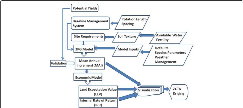
The signature feature of our approach was spatially explicit visualizations of potential profitability of target SRWC
spe-cies (Fig.1). For this we modeled productivity and potential
profitability at the spatial resolution of the 5-digit ZIP Code Tabulation Area (ZCTA) level in the operational range of each species. A ZCTA is generally smaller than a political sub-division such as a county but ZCTAs are not of uni-form area. For example, there are about 30,000 polygons averaging 16,900 ha each within the 38 states in the full BioSat system, although in the 13 southern states in the range of loblolly pine, the 10,016 ZCTAs average 20,900 ha each. Because demographic and other census data are col-lected and reported by ZCTAs, it was possible to combine socioeconomic with biophysical data in a common spatial
unit. We used the US ZCTA boundary map [85] to
com-bine model inputs and outputs for each ZCTA.
Geographic range
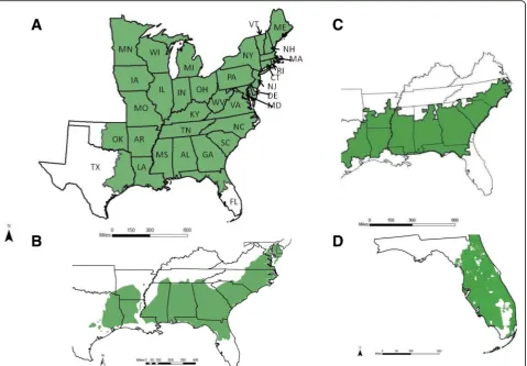
We identified the operational geographic range for each
of the species (Fig. 2). The ranges for the two native
species, Populus deltoides and Pinus taeda, were based
on Little [52].Eucalyptusspecies are not native to the USA
and are generally intolerant of cold weather, thus limited in their potential growing range in the southern USA. Of the
two non-native Eucalyptus species, E. grandis is grown
commercially in peninsular Florida and the operational
range was based on Rockwood [74]. E. benthamii is
thought to be adapted to the USDA Plant Hardiness Zones
9A and 9B [86], overlapping to some extent with the range
ofPinus taeda(Fig.2). It is one of theEucalyptusspecies
being grown in east Texas and west Louisiana [36].
Some areas were excluded because of higher value land use options than forestry. These were mostly coastal sites including Key West, St. Petersburg, Tampa, Hialeah, Ponce Inlet, Lauderdale, and Sea Hag Marina in peninsu-lar Florida; Panama City, Brooksville Chin, Apalachicola, Destin FT Walton, Jacksonville, and Ponce Inlet in the Florida panhandle; Charleston City in South Carolina; Freeport in Texas; Dauphin Island in Alabama; and Hack-berry in Louisiana.
Soil data
Tabular and spatial data for soil series were collected from
USDA Natural Resources Conservation Service [87]
SSURGO database at the county level. Each soil attribute was linked with the tabular component to acquire the attri-bute description and to determine its soil texture from NRCS Soil Series Description Query Facility. A matrix of soil texture classes (sand, sandy loam, clay loam, and clay) and associated fertility and soil water availability was
devel-oped to simplify inputs into 3PG (Table1). The matrix was
further divided into upland and lowland sites to represent differences in soil drainage; upland sites are moderately
Fig. 2Range maps of the five target species (aPopulus deltoides andP. hybrid;bPinus taeda;cEucalyptus benthamii;dEucalyptus grandis). (State abbreviations ALAlabama,ARArkansas,CTConnecticut,DEDelaware,FLFlorida,GAGeorgia,IAIowa,ILIllinois,INIndiana,KYKentucky,LALouisiana,MA Massachusetts,MDMaryland,MEMaine,MIMichigan,MNMinnesota,MOMissouri,MSMississippi,NCNorth Carolina,NHNew Hampshire,NJNew Jersey, NYNew York,OHOhio,OKOklahoma,PAPennsylvania,RIRhode Island,SCSouth Carolina,TNTennessee,TXTexas,VAVirginia,VT Vermont,WIWisconsin, WVWest Virginia)
Table 1Fertility rating, fertilizer response, minimum and maximum available soil water in terms of eight soil texture and site position combinations
Soil texture Site position Fertilityarating Fertilizerbresponse Minimumcavailable soil water Maximumcavailable soil water
Sand Upland 0.15 0.60 50 100
Sand Lowland 0.30 0.45 50 100
Sandy loam Upland 0.30 0.50 100 150
Sandy loam Lowland 0.50 0.30 100 150
Clay loam Upland 0.55 0.25 150 200
Clay loam Lowland 0.70 0.10 150 200
Clay Upland 0.65 0.15 200 250
Clay Lowland 0.75 0.05 200 250
a
Index of inherent soil fertility; 1 = high fertility, 0 = low fertility
b
Index of responsiveness to added nutrients that depends on ability to add leaf area
c
Available soil water in mm H20 m− 1
well- to exceptionally well-drained and lowland sites are somewhat poorly, poorly, and very poorly drained. The dominant texture class (soil texture with the largest area in a ZCTA) was assigned to each ZCTA using the spatial overlay feature of ArcGIS©.
To capture the range of productivity potential, we added
fertility and available soil moisture to the matrix (Table1).
The fertility rating is an index ranging from 0 to 1 where a
rating of“1”implies very high nutrient availability and“0”
frames the low end of available nutrition. The inherent fertility rating is based largely on how soil texture and soil organic matter affect soil nitrogen (and secondarily phos-phorus) supplying capacity and retention capacity. Avail-able soil water is a function of soil texture and depth; maximum and minimum available soil water was specified for each combination of texture class and site position; measurement units were millimeters of water depth per meter of soil depth. Available soil moisture was estimated
from texture as cm2m−1of soil depth (Table1).
Weather data
We acquired monthly mean data from 1995 to 2004 at regional weather stations in the operable range of each species. Monthly average data from individual weather
stations were obtained from NOAA [60]. Monthly
aver-aged solar radiation at each weather station location was
obtained from NASA [59]. Stations with incomplete
re-cords were excluded; for the counties with no data, we associated each one with the closest weather station with complete data. Weather data were collected at stations; hence there were some ZCTA with multiple data points. We derived monthly ZCTA-level weather data by aver-aging monthly data from each weather station within a ZCTA over the 10-year period from 1995 to 2004. The data input for a given month was the average of 10 monthly values for each weather variable.
Growth modeling
The target species differ in their growth habits and site requirements. Two of the target species are native to the eastern USA but differ considerably in their site
adapta-tions. Loblolly pine (Pinus taeda), an evergreen conifer,
is adapted to the climate and soils of the southern USA and is widely planted throughout the southern coastal
plain and Piedmont [80] and is the only one of the target
species that lacks the ability to coppice. Although all of
the other target species are broadleaves, the Populus
spp. are deciduous and theEucalyptusspecies are
ever-green. The other native species, Eastern cottonwood (Populus deltoides), grows best on better drained alluvial sites throughout the eastern states, achieving maximum
growth on riparian sites in the southern states [81].
Pop-lar hybrids have been developed that grow well in the northern states, outperforming the native cottonwood,
whereas cottonwood does better than hybrids in the
south due to better resistance to disease [55].
Conse-quently, we chose to model cottonwood and hybrid pop-lar differently; north of a dividing line along the border of Arkansas, Kentucky, Virginia, and Maryland, we
mod-eled hybrid poplar and cottonwood to the south [83].
The two non-nativeEucalyptus grandisandE.benthamii
are restricted in their potential range by cold
tempera-tures;E.grandisis the least frost tolerant of the two and
grown commercially in southern Florida. Somewhat
more frost tolerant, E. benthamii is thought to be
adapted to coastal plain sites farther north but not far
inland [82].
3PG model
The flexible 3PG model has been used successfully to es-timate productivity for a variety of sites and
environ-mental conditions [47], including greenfield situations
where the species had not previously been planted [1].
The values of some variables are likely specific to the
genetics of the species being used (e.g., [37, 93]) and
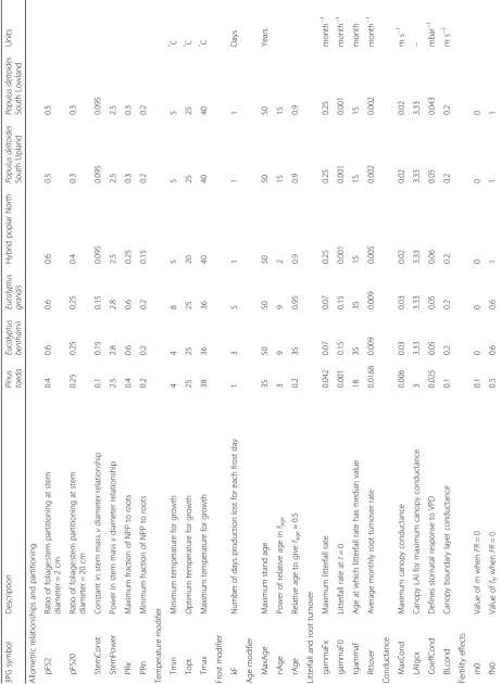
most work to date has used a combination of literature values and yield data from experimental treatments of fertilization, irrigation, or both to parameterize the model. We followed this approach and parameterized our model with the data available from multiple studies where the parameter values of interest may or may not have been the focus of the study. Model parameters used
for the target species are summarized in Table2.
The 3PG model estimates primary productivity for a species and then allocates that growth to various plant parts (roots, shoots, branches, and leaves). Approxi-mately 42 inputs are required to run the model. The pri-mary variables are detailed tree physiological measures and some are general constants or defaults typical of trees in general. Other variables are species-dependent: canopy structure and process variables (specific leaf area, extinction coefficient for photosynthetically active radi-ation absorption, age of full canopy cover, canopy quantum efficiency, and proportion of rainfall inter-cepted by canopy) determine light capture, light use, and precipitation interception.
Internal equations allocate NPP to the several tree com-ponents (bole, branches, and leaves, coarse and fine roots) . The portion of NPP allocated to the roots is influenced by moisture relations and soil nutrition. Allocations of NPP to stems and foliage are a function of the ratio of weight of foliage:dbh to the weight of stem:dbh. Foliage weight is impacted by soil nutrition, which is indexed by a fertility rating (FR) ranging from 0 to 1. Carbohydrate calculations are conducted on a single tree basis. Initial stand level stocking is a user-selected variable and survival is calculated using the self-thinning law. Litter fall and root turnover are calculated monthly.
SRWC species
Pinus taeda Loblolly pine has been modeled using 3PG
by Landsberg et al. [48] and Bryars et al. [14]. We used the
parameters from Bryars et al. [14] with only one exception,
a minor change in the TBB (age at which the branch and bark fraction equals one). The range is from age 0 to mature stands; they used 15 and we used 4 because of our
shorter rotation age [66].
Populus 3PG has been used to model growth of hybrid
poplar in Canada [3] and the northern USA [27,37]. We
used several parameters from Amichev et al. [3] directly
or as a base that was adjusted. Their study for hybrid
pop-lar Walker (P. deltoides×P.nigra) used data from three
sites in Saskatchewan, which is at the northern extreme of our region and their sites were planted at comparatively low densities. Because their values for canopy quantum efficiency, stem-foliage partitioning, and specific leaf area produced lower model estimates for the northern USA than validated production numbers for hybrid poplar in the literature, we adjusted parameter values for maximum canopy quantum efficiency, litterfall and root turnover,
and branch and bark fractions [3] but used their values for
specific gravity, temperature range, and the frost modifier. The 3PG model used for hybrid poplar was also used for
cottonwood [3] but some parameters varied slightly from
those used for hybrid poplar. The ratios of foliage:stem partitioning at two stem diameters, 2 and 20 cm (PFS2 and PFS20), were 0.5 and 0.3 for hybrid poplar versus 0.6 and
0.4 for P. deltoides. Optimal temperature for growth was
20 °C for hybrid poplar versus 25 °C forP. deltoides. The
coefficient of conductance, which defines stomatal response
to vapor pressure deficit, was set at 0.05 and 0.043 mbar−1
for P. deltoides on upland and lowland sites respectively
and 0.06 mbar−1 for hybrid poplar. Mainly due to initial
differences in planting density, maximum stem size per tree
was set at 220 kg tree−1forP.deltoidesand at 100 kg tree−1
for hybrid poplar.
Eucalyptus grandis andE.benthamii The 3PG model
has been used successfully to model various Eucalyptus
species [1, 29,46,76]. After comparing models developed
for E. grandis[1] and E. grandis× urophylla in Brazil [2,
29] and Dye et al. [29] for E. grandis ×camaldulensis in
South Africa, we based our work on Dye et al. [29]. Results
of the other two models were unrealistically high compared to literature and operational yields. We used the same
parameterization for both E. grandis and E. benthamii
except for the frost modifier, specific leaf area, and wood density.
The frost variables and modifiers in 3PG affect how monthly NPP is allocated. Frosts are infrequent in most of
the operational range ofE. grandis but they do occur so
we used a modifier of 5 days of production loss for each
frost day. For the less sensitive E. benthamii, the frost
modifier was set at 3 days per frost event. Estimates of
po-tential thresholds for foliage damage to E. benthamii by
age are based on observed damage [90] and the mortality
threshold is based on Dougherty and Wright [26]. A
higher value of specific leaf area (SLA) for E. benthamii,
9.1 m2kg−1was based on destructive sampling of
3-year-old trees near Fargo, GA (Dougherty, unpublished). A
higher value for wood density for E. benthamii of
0.55 g cm−3was based on Pirraglia et al. [70].
Initialization inputs
Initialization inputs describing site-specific values for soils included texture class, fertility effect, initial available soil water, and maximum and minimum available soil water
(Table1). Weather data included frost days, precipitation,
and minimum and maximum temperature. Species-specific data inputs included initial weights of foliage, stem, and root biomass, expected defoliation rates, and a
ranking for competition from weeds (Table2).
Silvicultural management regimes
We defined the silvicultural regimes for each species
(Table3). The genotypes used were those generally
avail-able to most producers so that the yields reflect current average genetic technology. Except for loblolly pine (bareroot), stock types for all species were cuttings. The management regime for each species was operationally intensive and aimed at advanced but economically feas-ible regimes. Planting density was the same for
cotton-wood and theEucalyptusspecies (1730 sph) and slightly
higher for loblolly pine (2224 sph). Hybrid poplar was planted at higher density, 10,000 sph, and managed
simi-larly to willow bioenergy systems (e.g., [88]).
size of the stump, the vigor of the harvested plant, and the internal allocation of carbohydrates at the time of harvest. Production increases in the initial coppice rotation and decreases in the second coppice stand be-cause mortality increases. We modeled the first coppice yield to be 115% of the initial harvest and a decline in the yield of the second coppice to 80% of the first coppice.
Poplars and eucalypts are capable of producing high leaf area levels resulting in high nutrient demand. Lob-lolly pine also exhibits rapid early growth and responds readily to fertilization. Growth across soil types de-pends on the ability to produce more leaf area for light interception. The response to fertilization depends on
the inherent (fertility rating in Table 1) or manipulated
level of soil fertility (fertility response). On soils with high inherent fertility, leaf area levels are already high and added nutrients will not increase light capture because it is already high. Alternatively, soils with inherently low nutrient levels can see major responses in productivity from fertilization because there is room to grow additional leaves for light capture. All stands were fertilized at rates comparable to current best prac-tices for economically viable biomass production for each species. Operational fertilization regimes typically include a starter fertilizer and one or more follow-up applications. Fertilization rates and other management
activities and their costs are given in Tables4,5, and6.
Validation
Our approach to model validation was to compare our modeled outputs to published or observed data for
lob-lolly pine, cottonwood and hybrid poplar, andE.grandis.
Normal practice would have been to completely parameterize the model on one set of data from a spe-cific site and then compare the modeled growth data to a second set of measured data. This was not appropriate since our interest was in mean yields over the geo-graphic ranges of the species. We did compare our data to literature results from field experiments and the pa-rameterizations we used were themselves validated in the usual way.
Economic modeling
A variety of approaches have been used to assess the
fi-nancial feasibility of SRWCs [31]; net present value
(NPV) is the most commonly used financial valuation method. This method discounts all costs and benefits over a rotation or a planning horizon to a reference time, i.e., it is the present value of future revenues minus the present value of future costs. The land expectation value (LEV) is the NPV of bare land assuming a perpet-ual land management regime and is used to correctly consider the opportunity cost of capital and land and
de-termine optimal forest management practices [17]. The
internal rate of return (IRR) of an investment is the dis-count rate at which the NPV equals zero. The higher a Table 3Silvicultural regimes for target woody crops in the eastern United States
Species Region Operable soilsa Planting density, trees ha−1
Initial rotation, years
Coppice rotations
Coppice length, years
Total rotation length, years
Pinus taeda Southeast S, SL, CL, C 2224 12 0 0 12
Populus deltoides South SL, CL, C 1730 8 2 8 24
HybridPopulus North SL, CL, C 10,005 4 5 4 24
Eucalyptus grandis South Florida S, SL, CL, C 1730 5 2 5 15
Eucalyptus benthamii Southeast S, SL, CL, C 1730 5 2 5 15
a
Soil textures:Ssandy,SLsilt loam,CLclay loam,Cclay
Table 4Management practices and related costs for loblolly pine (Pinus taeda) on lowlands and uplands (costs based on Dooley and Barlow [25])
Year Activity Bottomland Upland Cost, $US ha−1
0 Chemical site preparation X X 185
0 Spot pile, shear, and bed X 593
0 Di-ammonium phosphate application (22.4 kg ha−1) X X 89
0 Open pollinated seedlings (2224 trees ha−1) X X 124
0 Planting labor X X $178
0 Herbaceous weed control treatment X X 111
3 Urea Fertilizer (487.5 kg ha−1) X X 395
8
site’s IRR, the more desirable it is to plant the specific
SRWC species on the site. In our case, the“site”was the
ZCTA.
We used Microsoft Excel to estimate LEV and IRR for each species on each ZCTA within the operable range for the species, according to site conditions and published costs. The models focused on the cultivation phase of the SRWC species and excluded the cost of harvesting and transportation, as these costs would require specifying particular locations of conversion facilities. Model inputs included the mean annual increment (MAI) from the 3PG
model; site preparation costs, planting costs, fertilization costs, and stumpage biomass price were obtained from Timber Mart South, Timber Mart North, and state-level
reporting services (Tables4,5, and6); the LEV was
calcu-lated for each site using an annual discount rate of 5%. The IRR was also calculated using the cash flow of costs and revenues of the total rotation. The rotation length, the number of coppice rotations, and the ratios of initial and
coppice harvests were fixed for each species (Table3).
The models convert 3PG outputs, MAI of the volume
inside bark yield (m3ha−1 year−1), to weight of biomass
(Mg ha−1 year−1) using specific volume to dry weight
conversions (Table7). Considering that the yield given is
inside-bark biomass, the stumpage price was assumed to
be $10 Mg−1for all species, slightly higher than
Timber-Mart South pulpwood prices.
Visualization
To avoid the influence of the rigid shape of the ZCTA boundary, a second set of maps was produced with smooth boundaries using the Simple Kriging spatial interpolation technique implemented using ArcGIS®. The kriging method
has been widely used in soil science and geology [62], and
is considered the best linear unbiased estimator of the char-acteristic under study where it best reflects the minimum mean square error. It minimizes the variance of the estima-tion errors, resulting in a marked smoothing effect. The method assumed that the distance or direction between observed known points reflected a spatial correlation that can be used to explain variation in the surface. It uses a weighted moving average interpolation to produce the Table 5Management practices and related costs forEucalyptus
grandis and E.benthamii(costs based on Dooley and Barlow
[25])
Yeara Activity Cost, $US ha−1
0 Spot raking 99
0 Chemical site prep 161
0 Single pass bed 210
0 Weeding 86
0 Planting (1730 stems ha−1) 605
11 Weeding 124
11 Nitrogen fertilizer (45 kg ha−1) 96
22 Nitrogen fertilizer (179 kg ha−1) 388
44 Nitrogen fertilizer (224 kg ha−1) 484
55 Harvestb
0 Shearing (after each harvest) 222
a
Indicates the year of each rotation
b
Harvesting occurs at ages 5, 10, and 15
Table 6Management practices and related costs forPopulushybrids short-rotation woody biomass crops in the northern USA and
Populus deltoidesin the southern USA (costs based on Dooley and Barlow [25])
Year Activity Northern cost, $US ha−1 Southern cost, $US ha−1
0 Herbicide/weed control 267 111
0 Site prep 74 173
0 Mechanical tillage 111 161
0 Plantinga 2501 571
1 Herbicide/weed control 111
1 Nitrogen fertilizer (67 kg ha−1) 146
2 Nitrogen fertilizer (224 kg ha−1) 484
2 Nitrogen fertilizer (134 kg ha−1) 292
3 Nitrogen fertilizer (202 kg ha−1) 435
4 Harvestb X
0 Stump removal (after harvest) 741
6 Nitrogen fertilizer (180 kg ha−1) 435
8 Harvestc X
0 Stump removal (after harvest) $300
a
Planting hybrid poplar in the north is at 10,005 cuttings ha−1
; plantingP.deltoidesin the south is at 1730 cuttings ha−1 b
Harvesting occurs at ages 4, 8, 12, 16, 20, and 24 for hybrid poplar in the north
c
optimal spatial linear prediction. Mathematically, the form of the Simple Kriging estimator is
Zð Þ ¼μ mþX
nð Þμ
α¼1
λα½Zð Þμα −m μ;μ∝ ð1Þ
where μ, μ∝ are location vectors for estimation point
and one of the neighboring data points is indexed by
n(μ), the number of data points in local neighborhood
used for estimation of Z∗(μ); λα is an unknown weight
for the measured value at the pointα;mis the constant
and known expected value of Z∗(μα); and Z(μα) is the
known measured value of pointα. Unlike the weight,λα
is the IDW (inverse distance weighted), which depends solely on the distance to the prediction location; the
weight λα in the Kriging method is based not only on
the distance between the measured points and the pre-diction location but also on the overall spatial arrange-ment (or distribution) of the measured points.
Results
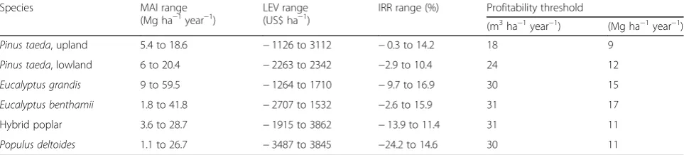
Production systems for SRWC are extremely regional-ized due to constraints imposed by species adaptation to key characteristics of soils and climate. Growth and pro-duction costs determine the potential for profitability based on acceptable mean annual increment (MAI), land expectation value (LEV), and internal rate of return (IRR). The ranges of modeled productivity, LEV, and IRR for the target species in the eastern USA are given in
Table8. Productivity was measured as mean annual
bio-mass increment (MAI; Mg ha−1year−1) or mean annual
volume increment (m3 ha−1 year−1) and was higher in
the southern portions of the ranges of each of the five
target species. Eucalyptus grandis in southern Florida
had the highest modeled biomass productivity
(59.5 Mg ha−1year−1). Yields ofE.grandiswere lower in
northern Florida given the prevalence of annual frost in
this region.Eucalyptus benthamiiis somewhat more
tol-erant of frost and can be planted farther north,
produ-cing potential yields almost as high as E. grandis. Both
species achieved positive LEV at similar volume growth
rates (30 and 31 m3 ha−1 year−1 for E. grandis and E.
benthamii, respectively; Table8).
Hybrid poplar in the northern states and Populus
del-toides in the southern states can also be quite productive with modeled potential volume productivity respectively, as
high as 31.6 and 29 m3 ha−1 year−1. While these species
have wide geographic ranges, indicating tolerance of a wide range of climates, they are also the most demanding of site and intolerant of low fertility and low available soil moisture [81].Pinus taeda(loblolly pine), the only conifer considered and the one species that does not coppice, is a widely planted commercial species in the southern USA. It had the highest potential biomass production in southeast Texas,
southwest Louisiana, and northern Florida [66]. Modeled
biomass increment was lower than the broadleaved species
with a maximum of 18.6 and 20.4 Mg ha−1year−1on
up-land and lowup-land sites, respectively.
Higher yields in the southern portion of the operable ranges of the five species also resulted in corresponding higher estimates of LEV and IRR. Return on invested capital was competitive for all five species; dependent on
the location of a species within its operable range.
Euca-lyptus benthamii had IRRs approaching 16% along the
coastal regions of the southern USA. Eucalyptus grandis
had IRR exceeding 20% in coastal regions of south
Flor-ida [82]. Hybrid poplar had IRR approaching 15% in
central Missouri, southern Indiana, and southern Illinois. Despite lower annual productivity than the other species, Pinus taeda nevertheless had an attractive IRR of ap-proximately 4% on uplands and apap-proximately 10% on lowlands. For the same soil texture, LEV and IRR for
Table 8Potential mean annual biomass increment (MAI), land expectation value (LEV), internal rate of return (IRR), and profitability threshold (minimum volume inside bark to yield LEV≥0) for target woody crops in the eastern United States
Species MAI range
(Mg ha−1year−1)
LEV range (US$ ha−1)
IRR range (%) Profitability threshold
(m3ha−1year−1) (Mg ha−1year−1)
Pinus taeda, upland 5.4 to 18.6 −1126 to 3112 −0.3 to 14.2 18 9
Pinus taeda, lowland 6 to 20.4 −2263 to 2342 −2.9 to 10.4 24 12
Eucalyptus grandis 9 to 59.5 −1264 to 1710 −9.7 to 16.9 30 15
Eucalyptus benthamii 1.8 to 41.8 −2707 to 1532 −2.6 to 15.9 31 17
Hybrid poplar 3.6 to 28.7 −1915 to 3862 −13.9 to 11.4 31 11
Populus deltoides 1.1 to 26.7 −3487 to 3845 −24.2 to 14.6 30 11
Table 7Volume to dry weight conversions for each species used in the biomass calculations
Species Volume to dry weight conversion
Pinus taeda 0.50
Eucalyptus benthamii 0.55
Eucalyptus grandis 0.50
Populus deltoides 0.35
loblolly pine were higher on uplands than on lowlands because of lower site preparation costs; although the projected yields on upland soils were generally lower
than those of lowland soils [66].
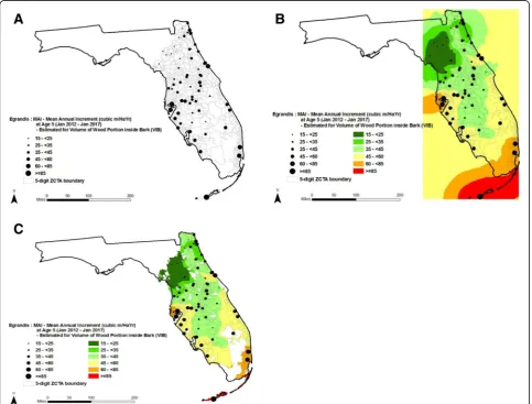
The kriging technique produced smoothed maps for
visu-alizing results and is illustrated with MAI results of E.
grandisin southern Florida, i.e., the volume yield estimates
for each ZCTA were used as input points (Fig. 3a). Five
neighboring points were included for calculating the kriging weights; a spherical semi-variogram was applied with default settings for a nugget of 2.35, a sill of 10.071, a range of 6.24 km, and a smoothing factor of 0.5. This produced a
rectangular raster map (Fig. 3b). That predictive map was
clipped to the range map to show the modeled volume
pro-duction (Fig.3c).
Discussion
Renewable energy has numerous technical, economic,
and social challenges [79], one of which is the availability
of sustainable biomass feedstock. The renewed interest in the USA in fast growing trees for bioenergy
planta-tions [69] has raised a number of questions as to
sus-tainability, carbon neutrality, and effects on biodiversity
[41,84] as well as economic feasibility [33,56].
Answer-ing these questions requires site- and species-specific information; this study begins to address these problems by developing spatially specific SRWC data on growth potential and economic analyses. Additionally, these data provide a coarse filter for practitioners interested in siting biomass facilities.
The modeled biomass growth potential of four species and one hybrid, validated against existing data, literature, on-going research, and expert guidance, indicated that a SRWC feedstock supply chain system is likely to be highly affected by local biophysical characteristics governing the productivity potential of the species being considered. The analysis is based on baseline management systems and in-puts that can be modified in alternative management
systems for each species. Profitability potential was de-rived from the productivity estimates using standard eco-nomic analyses (LEV and IRR). Analyses and visualization of results was done at the spatial resolution of the 5-digit
ZIP Code Tabulation Area level (Figs. 1 and 2); each
5-digit ZCTA is unique in terms of species suitability, cost, and productive potential. The spatial resolution of the ZCTA is higher than administrative units such as counties and much other socioeconomic data are available at the ZCTA-level for further analysis such as the impact of
natural hazards on biomass supply chains [64].
A detailed economic and comparative analysis is feasible between the target species where ranges overlap. Any incentives, such as payments for ecological services or sub-sidies, which would add value for growing biomass, could also increase SRWC production at a particular location. Assessing ecological service from properly designed and managed SRWC would benefit from the explicit spatial
information from our method [19,92,94,95].
The biomass yield numbers can be used for further economic evaluation, carbon sequestration studies, phy-totechnologies, and sustainability research. Potential en-vironmental effects of widespread deployment of SRWC could use our spatially explicit results to focus analysis and inform potential debate. In particular, the renewed
interest in planting frost-tolerantEucalyptus species,
in-cluding genetically modified organisms, beyond southern Florida has aroused concerns for adverse effects on bio-diversity, water supply, and potential extreme fire behavior
[35, 54,82,89] and realistic assessments of potential
prob-lems require knowing where plantings would be
economic-ally feasible, as found in Stanturf et al. [82]. Our results
indicate that future deployment ofE.benthamiiwill remain
constrained to coastal areas due to growth reductions from
episodic low temperatures and frost; Wear et al. [89] suggest
that even genetically modified freeze-tolerant Eucalyptus
will be limited by market uncertainties despite the potential
to meet shortfalls in supply of hardwood fiber [43].
Growth potential was assessed at the landscape-scale, which is insufficient for assessing actual biomass supply levels. The growth and yield models that could provide this
information are available for Pinus taeda and to a lesser
extent for hybrid poplar but not so for the other target species and there is insufficient empirical data to evaluate all combinations of site, climate, and management systems. More detailed assessments could use our results as a coarse filter to look either at where to locate a dedicated bioenergy facility or to evaluate the potential for a developed site to utilize one of the target species to produce bioenergy, followed by more detailed analysis using available empirical data and models.
Our method has some limitations that can be over-come or mitigated by further research and development. Continued research to further frame the parameters for
the 3PG model is needed, for these target species as well as
other species of interest such asPlatanus occidentalis
(syca-more) and Liquidambar styraciflua(sweetgum) that have
been suggested for SRWC [42,69]. The 3PG model itself
could be improved. The variables for canopy structure and
processes (Table2) are particularly important as they define
the light use efficiency, defining light interception as well as carbon capture by the canopy. The canopy quantum effi-ciency variable specifically is an estimate of the production of carbon produced per unit of light captured. Small changes in this parameter result in substantial changes in the estimated productivity, other factors held constant. The difference in value of this parameter for the species
consid-ered is apparent; it was greatest for theEucalyptusspecies,
slightly less for Populus spp., and least for Pinus taeda.
Other variables are sensitive to the choice of species as well, particularly specific leaf area and the suite of variables that define canopy conductance. Improved parameterization of phenology and biomass partitioning emphasizing clonal
differences would be especially helpful [94].
This modeling framework can be extended to other questions such as the effects of extreme weather and cli-mate change, as well as carbon substitution and seques-tration potential of SRWC. Our weather inputs were limited to a 10-year interval, sufficient to run the model but did not incorporate the effects of weather extremes. A few drought years could significantly lower productiv-ity and therefore profitabilproductiv-ity. The 3PG model is flexible and could incorporate weather scenarios to assess risk of failure or lowered yields. Coupling the model to future weather scenarios from climate models would allow for spatially explicit estimates of climate change effects such
as from extreme weather [12,75]. Because of the linkage
of land cover types to climate, using this framework to model realistic widespread deployment of SRWC that converted agricultural land would provide indications of
their effects on climate (e.g., [13,18,53]).
We used specific silvicultural and management regimes for each target species, based on standard practices. Lower costs under different regimes might extend profitability to more sites; other management options might increase
income. The well-developed value chain forPinus taedain
the US South, for example, could allow for other biomass/ bioenergy combinations such as interplanting with an herbaceous bioenergy crop or a dual-cropping system with
sawlog or pulpwood and bioenergy [66]. The very
high-density system we used for hybrid poplar in the northern half of the eastern USA was non-standard; other work has
examined more traditional spacing [37, 49, 93] and we
wished to avoid duplication. In the northeastern USA,
high-density Salix bioenergy systems are under
develop-ment [88, 92] and we sought results that could be
[88]; our hybrid poplar results are well-within this range
(Table8).
Conclusions
Economic variations impact public, private, or venture-backed biomass businesses in many different ways. Gener-ally, biomass supply systems are hindered by a lack of geographical specificity of feedstock supply. Assessing the economic feasibility and sustainability of biomass supply is essential for this emerging industry. The US Billion-Ton
Update report [69] projected that more cellulosic feedstock
will be available at higher feedstock prices. Increasing the available feedstock by lowering cost, increasing productiv-ity, and stabilizing logistics would have the same effect as higher feedstock prices. A species production cost and its corresponding market price will likely influence the feedstock selected for inclusion in the biomass supply chain. The feedstock market price will also affect the size of an area where it is likely to be deployed, imply-ing that productive potential and species type and gen-etics are the important factors determining locations
for conversion facilities [49].
This study provides value for the emerging bio-economy by estimating yields and return on investments at the resolution of the 5-digit ZCTA for target species
in the Eastern USA: Pinus taeda, Populus deltoidesand
hybrids, Eucalyptus grandis, and Eucalyptus benthamii.
The key findings in our analysis are:
1. Local characteristics (site and climate) governing the productivity potential of a species being considered for a SRWC feedstock supply chain system determines potential profitability 2. Regional analyses of productivity and potential
profitability of SRWC can be accomplished using a process-based model such as 3PG
3. Biomass yields as measured in mean annual biomass increment (Mg ha−1year−1) were higher in the southern portions of the operable ranges of each of the four target species
4. Eucalyptus grandisin southern Florida had the highest modeled productivity (59.5 Mg ha−1year−1) 5. Return on invested capital was competitive for all
four species but depended highly on the location within its operable range
6. This modeling framework can be extended to other questions such as the effects of extreme weather and climate change, carbon substitution and sequestration potential of SRWC, and potential environmental effects of widespread deployment of SRWCs including non-nativeEucalyptusspecies.
Abbreviations
IRR:Internal rate of return; LEV: Land expectation value; MAI: Mean annual increment; ZCTA: Zip code tabulation area
Acknowledgements
We thank numerous anonymous reviewers for valuable comments that helped improve the paper. The authors also acknowledge the University of Tennessee Agricultural Experiment Station, Center for Renewable Carbon, and Department of Forestry, Wildlife and Fisheries and the US Forest Service Southern Research Station Center for Forest Disturbance Science. Soils data were obtained from the Soil Survey Staff, Natural Resources Conservation Service, United States Department of Agriculture, Web Soil Survey. Weather data were obtained from the NOAA National Centers for Environmental Information (formerly the National Climatic Data Center). Solar radiation data were provided by the NASA Langley Research Center Atmospheric Science Data Center Surface Meteorological and Solar Energy (SSE) web portal supported by the NASA LaRC POWER Project. During the research, Stanturf was with the US Forest Service.
Authors’contributions
JAS—Lead: site suitability, ecological parameters, and growth modeling (3PG); JHP—Overall lead: study design, coordination, and oversight; supply chain analytics; TMY—Lead: statistical algorithms and data fusion, logistic regression analysis and spatial correlation and SQL database-GIS integration within BioSAT. XH—Statistics, GIS analysis and mapping, visualization, and data techniques; ZG—economic modeling, MAI, LEV, IRR. DD and MP—3-PG Model and yield outputs for SRWC species. All authors read and approved the final manuscript.
Authors’information
The lead authors’expertise and research credentials provided an opportunity to contribute to a national energy strategy that produced four unified studies, namely the 2005 US Billion-Ton Study (BTS), the 2011 U.S. Billion-Ton Update (BT2), and the 2016 US Billion-Ton Report, Volume 1 and 2. J. H. Perdue is a retired senior biological scientist supporting biobased research to achieve economic prosperity and ecological benefits with the USDA Forest Service, Center for Forest Disturbance Science. He earned Natural Resource and Forestry degrees from Colorado State University, Auburn University and Wallace State Community College. His capability has taken him across the USA leading complex projects in natural resource risk management and policy; financial and resource evaluation; and economic development. Currently, he leverages and advances a multi-partner research collaborative deploying innovative biomass and bioenergy decision support and visualization tools. The tools make use of socio-economic and biophys-ical drivers as well as the place-based human-environmental conditions that influence biobased land-use decisions. During his career, he has accumulated an outstanding slate of recognition including: Council on Environmental Quality Award for Excellence in Environmental Planning; Innovator of the Year Award from the Southern Governors and numerous awards for National and Regional biobased leadership.
J. A. Stanturf is a Visiting Professor, Institute of Forestry and Rural
Fulbright Professorat Salzburg University of Applied Sciences in Austria in 2013 and a Fulbright Specialist in Austria in 2016. He received the“Alumni of the Year”award in 2018 from the University of Wisconsin, Madison. He is an active member and past President of the Forest Products Society (FPS) and active in the American Society of Quality (ASQ), American Statistical Associ-ation (ASA).
Funding
Direct support for this research project was primarily from the U.S. Forest Service, Southern Research Station, including research agreement FS 07CR11330115087 to the University of Tennessee. Other support included USDA Southeastern Sun Grant Center, and USDA McIntire-Stennis research project TENOOMS-101. The authors had financial support from The University of Tennessee Agricultural Experiment Station, Center for Renewable Carbon, and Department of Forestry, Wildlife and Fisheries.
Availability of data and materials Data available upon request.
Ethics approval and consent to participate Not applicable.
Consent for publication Not applicable.
Competing interests
The authors declare that they have no competing interests.
Author details
1Estonian University of Life Sciences, Tartu, Estonia.2U.S. Forest Service,
Southern Research Station, Knoxville, TN, USA.3Center for Renewable Carbon, The University of Tennessee, Knoxville, TN, USA.4Dougherty & Dougherty Forestry Services, Inc, Danielsville, GA, USA.
Received: 11 March 2019 Accepted: 21 June 2019
References
1. Almeida AC, Landsberg JJ, Sands PJ (2004) Parameterisation of 3-PG model for fast-growingEucalyptus grandisplantations. For Ecol Manag 193:179–195 2. Almeida AC, Siggins A, Batista TR, Beadle C, Fonseca S, Loos R (2010)
Mapping the effect of spatial and temporal variation in climate and soils on Eucalyptusplantation production with 3-PG, a process-based growth model. For Ecol Manag 259:1730–1740
3. Amichev BY, Johnston M, Van Rees KC (2010) Hybrid poplar growth in bioenergy production systems: biomass prediction with a simple process-based model (3PG). Biomass Bioenergy 34:687–702
4. Badger P (2002) Processing cost analysis for biomass feedstock. Prepared for the US Department of Energy. Under contract DE-AC05-00OR22725 ORNL/ TM-2002/199; Oak Ridge National Laboratory, TN
5. Badger PC, Fransham P (2006) Use of mobile fast pyrolysis plants to densify biomass and reduce biomass handling costs—a preliminary assessment. Biomass Bioenergy 30:321–325
6. Benjamin J, Lilieholm RJ, Damery D (2009) Challenges and opportunities for the northeastern forest bioindustry. J For 107:125–131
7. Bennich T, Belyazid S (2017) The route to sustainability—prospects and challenges of the bio-based economy. Sustainability 9(6):887https://doi.org/ 10.3390/su9060887
8. BioSAT (2012) The BioSAT Project.http://www.biosat.net/. Accessed 4 Mar 2019
9. Birdsey R, Duffy P, Smyth C, Kurz WA, Dugan AJ, Houghton R (2018) Climate, economic, and environmental impacts of producing wood for bioenergy. Environ Res Lett 13(5):050201https://doi.org/10.1088/1748-9326/aab9d5
10. Birner R (2018) Bioeconomy concepts. In: Lewandowski I (ed) Bioeconomy. Springer Open, pp 17–38https://doi.org/10.1007/978-3-319-68152-8_2
11. Bracco S, Calicioglu O, Gomez San Juan M, Flammini A (2018) Assessing the contribution of bioeconomy to the total economy: a review of national frameworks. Sustainability 10(6):1698https://doi.org/10.3390/su10061698
12. Breuer H, Ács F, Skarbit N (2018) Observed and projected climate change in the European region during the twentieth and twenty-first centuries according to Feddema. Clim Chang 150:377–390
13. Bright RM, Zhao K, Jackson RB, Cherubini F (2015) Quantifying surface albedo and other direct biogeophysical climate forcings of forestry activities. Glob Chang Biol 21:3246–3266
14. Bryars C, Maier C, Zhao D, Kane M, Borders B, Will R, Teskey R (2013) Fixed physiological parameters in the 3-PG model produced accurate estimates of loblolly pine growth on sites in different geographic regions. For Ecol Manag 289:501–514
15. Carmenza R-A et al (2017) Bioenergy production and sustainable development: science base for policymaking remains limited GCB. Bioenergy 9:541–556
16. Carus M (2017) Biobased economy and climate change—important links, pitfalls, and opportunities. Ind Biotechnol 13:41–51
17. Chang SJ (1998) A generalized Faustmann model for the determination of optimal harvest age. Can J For Res 28:652–659
18. Chen G-S, Notaro M, Liu Z, Liu Y (2012) Simulated local and remote biophysical effects of afforestation over the southeast United States in boreal summer. J Clim 25:4511–4522
19. Coleman MD, Stanturf JA (2006) Biomass feedstock production systems: economic and environmental benefits. Biomass Bioenergy 30:693–695 20. Cornwall W (2017) Is wood a green source of energy? Scientists are divided.
Science 355:18–21
21. Dale VH et al (2017a) Status and prospects for renewable energy using wood pellets from the southeastern United States GCB. Bioenergy 9:1296–1305 22. Dale VH, Parish E, Kline KL, Tobin E (2017b) How is wood-based pellet production affecting forest conditions in the southeastern United States? For Ecol Manag 396:143–149
23. Dauvergne P, Neville KJ (2010) Forests, food, and fuel in the tropics: the uneven social and ecological consequences of the emerging political economy of biofuels. J Peasant Stud 37:631–660
24. Demirbas A (2009) Biofuels: securing the planet’s future energy needs. Energy Convers Manag 50(9):2239–2249
25. Dooley E, Barlow R (2013) Costs and trends of southern forestry practices 2012. Alabama Cooperative Extension System, Auburn
26. Dougherty D, Wright J (2012) Silviculture and economic evaluation of eucalypt plantations in the Southern US. BioResources 7:1994–2001 27. Dowell RC, Gibbins D, Rhoads JL, Pallardy SG (2009) Biomass production
physiology and soil carbon dynamics in short-rotation-grownPopulus deltoidesandP. deltoides×P. nigrahybrids. For Ecol Manag 257:134–142 28. Duden AS et al (2017) Modeling the impacts of wood pellet demand on forest dynamics in southeastern United States. Biofuels Bioprod Biorefin 11: 1007–1029
29. Dye P, Jacobs S, Drew D (2004) Verification of 3-PG growth and water-use predictions in twelve Eucalyptus plantation stands in Zululand, South Africa. For Ecol Manag 193:197–218
30. Efroymson RA et al (2017) 2016 billion-ton report: advancing domestic resources for a thriving bioeconomy, volume 2: environmental sustainability effects of select scenarios from volume 1. Oak Ridge National Lab., Oak Ridge; Argonne National Lab, Lemont
31. El Kasmioui O, Ceulemans R (2012) Financial analysis of the cultivation of poplar and willow for bioenergy. Biomass Bioenergy 43:52–64
32. Fargione J, Hill J, Tilman D, Polasky S, Hawthorne P (2008) Land clearing and the biofuel carbon debt. Science 319:1235–1238
33. Ghezehei SB, Shifflett SD, Hazel DW, Nichols EG (2015) SRWC bioenergy productivity and economic feasibility on marginal lands. J Environ Manag 160:57–66 34. Golden JS, Handfield R, Pascual-Gonzalez J, Agsten B, Brennan T, Khan L,
True E (2018) Indicators of the US biobased economy. United States Department of Agriculture, Office of the Chief Economist, Washington DC 35. Goodrick SL, Stanturf JA (2012) Evaluating potential changes in fire risk from
eucalyptus plantings in the southern United States. Int J For Res 2012:9.
https://doi.org/10.1155/2012/680246
36. Hart PW, Santos RB (2015) Changing the face of short fiber-a review of the Eucalyptus revolution. TAPPI J 14:353–359
37. Headlee WL, Zalesny RS, Donner DM, Hall RB (2013) Using a process-based model (3-PG) to predict and map hybrid poplar biomass productivity in Minnesota and Wisconsin, USA. BioEnergy Res 6:196–210
38. Henderson JE, Joshi O, Parajuli R, Hubbard WG (2017) A regional assessment of wood resource sustainability and potential economic impact of the wood pellet market in the US South. Biomass Bioenergy 105:421–427 39. Hinchee M et al (2009) Short-rotation woody crops for bioenergy and
40. Huang X, Perdue JH, Young TM (2012) A spatial index for identifying opportunity zones for woody cellulosic conversion facilities. Int J For Res 2012:106474, 11 pages.https://doi.org/10.1155/2012/106474
41. Immerzeel DJ, Verweij PA, Van Der Hilst F, Faaij AP (2014) Biodiversity impacts of bioenergy crop production: a state-of-the-art review. GCB Bioenergy 6:183–209 42. Johnson JM, Coleman MD, Gesch R, Jaradat A, Mitchell R, Reicosky D,
Wilhelm W (2007) Biomass-bioenergy crops in the United States: a changing paradigm. Am J Plant Sci Biotech 1(1):1–28
43. Kellison R, Lea R, Marsh P (2013) Introduction of Eucalyptus spp. into the United States with special emphasis on the southern United States. Int J For Res 189393:1–9https://doi.org/10.1155/2013/189393
44. Kim S, Dale BE (2015) All biomass is local: the cost, volume produced, and global warming impact of cellulosic biofuels depend strongly on logistics and local conditions. Biofuels Bioprod Biorefin 9:422–434
45. Kirschbaum MU (2003) To sink or burn? A discussion of the potential contributions of forests to greenhouse gas balances through storing carbon or providing biofuels. Biomass Bioenergy 24:297–310
46. Landsberg J, Waring R (1997) A generalised model of forest productivity using simplified concepts of radiation-use efficiency, carbon balance and partitioning. For Ecol Manag 95:209–228
47. Landsberg J, Waring R, Coops N (2003) Performance of the forest productivity model 3-PG applied to a wide range of forest types. For Ecol Manag 172:199–214
48. Landsberg JJ, Johnsen KH, Albaugh TJ, Allen HL, McKeand SE (2001) Applying 3-PG, a simple process-based model designed to produce practical results, to data from loblolly pine experiments. For Sci 47:43–51 49. Lazarus W, Headlee WL, Zalesny RS (2015) Impacts of supplyshed-level
differences in productivity and land costs on the economics of hybrid poplar production in Minnesota, USA. BioEnergy Res 8:231–248 50. Langholtz MH et al (2016) 2016 billion-ton report: advancing domestic
resources for a thriving bioeconomy, volume 1: economic availability of feedstocks. Oak Ridge National Lab.(ORNL), Oak Ridge
51. Lewandowski I (2017) Bioeconomy: shaping the transition to a sustainable, biobased economy. Springer Open, Cham
52. Little EL Jr (1971) Atlas of United States trees, vol. 1 Conifers and important hardwoods USDA Forest Service Miscellaneous Publication 1146, Washington DC
53. Liu Y, Stanturf J, Lu H (2008) Modeling the potential of the northern China forest shelterbelt in improving hydroclimate conditions. J Am Water Resour Assoc 44:1176–1192
54. Maier CA et al (2017) Comparative water use in short-rotationEucalyptus benthamiiandPinus taedatrees in the Southern United States. For Ecol Manag 397:126–138
55. Maisenhelder L (1970) Eastern cottonwood selections outgrow hybrids on southern sites. J For 68:300–301
56. McKenney DW, Weersink A, Allen D, Yemshanov D, Boyland M (2014) Enhancing the adoption of short rotation woody crops for bioenergy production. Biomass Bioenergy 64:363–366
57. Metzner C, Platzer M, Young TM, Bichescu B, Barbu MC, Rials TG (2019) Accurately estimating and improving costs for the cellulosic biomass supply chain with statistical process control and the Taguchi loss function. BioResources 14(2):2961–2976
58. Möller B, Nielsen PS (2007) Analysing transport costs of Danish forest wood chip resources by means of continuous cost surfaces. Biomass Bioenergy 31: 291–298
59. NASA (2015) Atmospheric science data center. Surface meteorology and solar energy [Data file].https://power.larc.nasa.gov/. Accessed 12 July 2015 60. NOAA (2012) National Climatic Data Center. Local weather observation
station record [Data file].https://www.ncdc.noaa.gov/cdo-web/. Accessed 12 July 2015
61. Olesen AS, Bager S, Kittler B, Price W, Aguilar F (2016) Environmental implications of increased reliance of the EU on biomass from the South East US European Commission Report ENV.B.1/ETU/2014/0043, European Commission, Brussels
62. Oliver MA, Webster R (1990) Kriging: a method of interpolation for geographical information systems. Int J Geogr Inf Syst 4:313–332 63. Openshaw K (2010) Biomass energy: employment generation and its
contribution to poverty alleviation. Biomass Bioenergy 34:365–378 64. Perdue JH, Stanturf JA, Young TM, Huang X (2019) A geospatial biomass
supply model adjusted for risk for natural disasters. Scand J For Res:1–32
https://doi.org/10.1080/02827581.2019.1587500
65. Perdue JH, Young TM, Rials TG (2011) The biomass site assessment model—BioSAT, Final Report for U.S. Forest Service, Southern Research Station submitted by The University of Tennessee, Knoxville, p 282 66. Perdue JH, Stanturf JA, Young TM, Huang X, Dougherty D, Pigott M, Guo Z
(2017) Profitability potential forPinus taedaL. (loblolly pine) short-rotation bioenergy plantings in the southern USA. Forest Policy Econ 83:146–155 67. Perez-Verdin G, Grebner DL, Sun C, Munn IA, Schultz EB, Matney TG (2009)
Woody biomass availability for bioethanol conversion in Mississippi. Biomass Bioenergy 33:492–503
68. Perlack RD (2005) Biomass as feedstock for a bioenergy and bioproducts industry: the technical feasibility of a billion-ton annual supply. Oak Ridge National Laboratory, Oak Ridge
69. Perlack RD et al (2011) US billion-ton update: biomass supply for a bioenergy and bioproducts industry. Oak Ridge National Laboratory, Oak Ridge 70. Pirraglia A, Gonzales R, Saloni D, Wright J, Denig J (2011) Fuel properties
and suitability of Eucalyptus benthamii andEucalyptus macarthuriifor torrefied wood and pellets. BioResources 7:0217–0235
71. Reijnders L (2006) Conditions for the sustainability of biomass based fuel use. Energy Policy 34:863–876
72. Righelato R, Spracklen DV (2007) Carbon mitigation by biofuels or by saving and restoring forests? Science 317:902–902
73. Robertson GP et al (2008) Sustainable biofuels redux. Science 322:49–50 74. Rockwood DL (2012) History and status of Eucalyptus improvement in Florida.
Int J For Res 2012:607879, 10 pages.https://doi.org/10.1155/2012/607879
75. Rummukainen M (2012) Changes in climate and weather extremes in the 21st century. Wiley Interdiscip Rev Clim Chang 3:115–129
76. Sands P, Landsberg J (2002) Parameterisation of 3-PG for plantation grown Eucalyptus globulus. For Ecol Manag 163:273–292
77. Schelhas J, Hitchner S, Brosius JP (2018) Envisioning and implementing sustainable bioenergy systems in the US South. In: Filho WL, Marans RW, Callewaert J (eds) Handbook of sustainability and social science research. Springer, Cham, pp 301–314
78. Schlesinger WH (2018) Are wood pellets a green fuel? Science 359:1328– 1329
79. Smith CT, Lattimore B, Berndes G, Bentsen NS, Dimitriou I, Langeveld JWA, Thiffault E (2017) Opportunities to encourage mobilization of sustainable bioenergy supply chains. Wiley Interdiscip Rev 6:e237https://doi.org/10.1002/wene.237
80. Stanturf JA, Kellison RC, Broerman FS, Jones SB (2003) Productivity of southern pine plantations: where are we and how did we get here? J For 101:26–31 81. Stanturf JA, Van Oosten C, Netzer DA, Coleman MD, Portwood CJ (2001)
Ecology and silviculture of poplar plantations. In: Dickmann DI, Isebrands JG, Eckenwalder JE, Richardson J (eds) Poplar culture in North America. NRC Research Press Canada, Ottawa, pp 153–206
82. Stanturf JA, Young TM, Perdue JH, Dougherty D, Pigott M, Guo Z, Huang X (2018) Productivity and profitability potential for non-native Eucalyptus plantings in the southern USA. Forest Policy Econ 97:210–222
83. Stanturf JA, Young TM, Perdue JH, Doughetry D, Pigott M, Guo Z, Huang X (2017) Potential profitability zones for Populus spp. biomass plantings in the eastern United States. For Sci 63:586–595
84. Tarr NM, Rubino MJ, Costanza JK, McKerrow AJ, Collazo JA, Abt RC (2017) Projected gains and losses of wildlife habitat from bioenergy-induced landscape change. GCB Bioenergy 9:909–923
85. US Census Bureau (2010) ZIP Code™Tabulation Areas( ZCTAs™)https:// www.census.gov/programs-surveys/geography/guidance/geo-areas/zctas. html. Accessed 12 Feb 2016
86. USDA ARS (2012) Plant hardiness zones maphttps://planthardiness.ars.usda. gov/PHZMWeb/. Accessed 12 Feb 2016
87. USDA Natural Resources Conservation Service (2012) SSURGO database soil survey [data file];https://sdmdataaccess.nrcs.usda.gov/. Accessed 12 July 2015 88. Volk T et al (2011) Yields of willow biomass crops across a range of sites in
North America. Asp Appl Biol 112:67–74
89. Wear DN, Dixon E, Abt RC, Singh N (2015) Projecting potential adoption of genetically engineered freeze-tolerant Eucalyptus in the United States. For Sci 61:466–480
90. Wright L, Eaton L, Perlack B (2010) Published and reported woody crop biomass yield data. Presented at October 19, 2010 SRWCOWG Meeting, Oak Ridge, TN 91. Young TM, Zaretzki RL, Perdue JH, Guess FM, Liu X (2011) Logistic
regression models of factors influencing the location of bioenergy and biofuels plants. BioResources 6(1):329–343
X, Pan X (eds) Sustainable production of fuels, chemicals, and fibers from forest biomass. ACS Symposium Series Volume 1067, American Chemical Society, Washington DC, pp 27–63
93. Zalesny RS Jr, Donner DM, Coyle DR, Headlee WL (2012) An approach for siting poplar energy production systems to increase productivity and associated ecosystem services. For Ecol Manag 284:45–58
94. Zalesny RS et al (2016a) Environmental technologies of woody crop production systems. BioEnergy Res 9:492–506.https://doi.org/10.1007/ s12155-016-9738-y
95. Zalesny RS et al (2016b) Ecosystem services of woody crop production systems. BioEnergy Res 9:465–491.https://doi.org/10.1007/s12155-016-9737-z
Publisher’s Note

![Table 5 Management practices and related costs for Eucalyptusgrandis and E. benthamii (costs based on Dooley and Barlow[25])](https://thumb-us.123doks.com/thumbv2/123dok_us/324169.1524889/10.595.59.539.496.707/table-management-practices-related-eucalyptusgrandis-benthamii-dooley-barlow.webp)