Application of genetic algorithms and constructive neural networks for the analysis of microarray cancer data

R E S E A R C H

Open Access

Application of genetic algorithms and

constructive neural networks for the analysis of

microarray cancer data

Rafael Marcos Luque-Baena

, Daniel Urda

, Jose Luis Subirats

, Leonardo Franco

, Jose M Jerez

From

1st International Work-Conference on Bioinformatics and Biomedical Engineering-IWBBIO 2013

Granada, Spain. 18-20 March 2013

* Correspondence: rmluque@lcc. uma.es

1_{Department of Computer Science,}

University of Málaga, Málaga, Spain

Abstract

Background:Extracting relevant information from microarray data is a very complex task due to the characteristics of the data sets, as they comprise a large number of features while few samples are generally available. In this sense, feature selection is a very important aspect of the analysis helping in the tasks of identifying relevant genes and also for maximizing predictive information.

Methods:Due to its simplicity and speed, Stepwise Forward Selection (SFS) is a widely used feature selection technique. In this work, we carry a comparative study of SFS and Genetic Algorithms (GA) as general frameworks for the analysis of microarray data with the aim of identifying group of genes with high predictive capability and biological relevance. Six standard and machine learning-based

techniques (Linear Discriminant Analysis (LDA), Support Vector Machines (SVM), Naive Bayes (NB), C-MANTEC Constructive Neural Network, K-Nearest Neighbors (kNN) and Multilayer perceptron (MLP)) are used within both frameworks using six free-public datasets for the task of predicting cancer outcome.

Results:Better cancer outcome prediction results were obtained using the GA framework noting that this approach, in comparison to the SFS one, leads to a larger selection set, uses a large number of comparison between genetic profiles and thus it is computationally more intensive. Also the GA framework permitted to obtain a set of genes that can be considered to be more biologically relevant. Regarding the different classifiers used standard feedforward neural networks (MLP), LDA and SVM lead to similar and best results, while C-MANTEC and k-NN followed closely but with a lower accuracy. Further, C-MANTEC, MLP and LDA permitted to obtain a more limited set of genes in comparison to SVM, NB and kNN, and in particular C-MANTEC resulted in the most robust classifier in terms of changes in the parameter settings.

Conclusions:This study shows that if prediction accuracy is the objective, the GA-based approach lead to better results respect to the SFS approach, independently of the classifier used. Regarding classifiers, even if C-MANTEC did not achieve the best overall results, the performance was competitive with a very robust behaviour in terms of the parameters of the algorithm, and thus it can be considered as a candidate technique for future studies.

Introduction

DNA microarray technology has been widely used in cancer studies for prediction of disease outcome [1]. It is a powerful platform successfully used for the analysis of gene expression in a wide variety of experimental studies [2]. However, due to the large number of features (in the order of thousands) and the small number of samples (mostly less than a hundred) in this kind of datasets, microarray data analysis faces the “large-p-small-n” paradigm [3] also known as the curse of dimensionality. In this sense, feature selection preprocessing refers to decide which genes to include in the prediction, and it is a crucial step in developing a class predictor. Including too many features could reduce the model accuracy and may lead to overfit the data [4]. Two different algorithms have been widely used in literature to carry out feature selection, the Stepwise Forward Selection algorithm (SFS) and the Genetic Algorithms (GA). In the SFS algorithm the choice of predictive features is carried out by an automatic pro-cedure that starts from single variable models and tests the addition of each feature using a comparison criterion. This algorithm has been used to identify a predictive gene signature whose size is minimum [5,6]. GA are also well considered as suitable evolutionary strategies for feature selection in problems with a large number of fea-tures [7,8], and are applied to different areas, from object detection [9] to gene selec-tion in microarray data [10].

On the other hand, model selection is another important step in the estimation of expression profiles to predict diseases outcome[11]. In this regards, different well-known machine learning-based techniques have been used recently in literature wrapped into features selection algorithms to develop a class predictor, e.g. Support Vector Machines (SVM)[12], Multilayer Perceptron (MLP)[13], k-Nearest Neighbor-hood (kNN)[14], Linear Discriminant Analysis (LDA)[15] and NaiveBayes. Neverthe-less, few of these related works brings together different learning algorithms, features selection schemes and input datasets. Besides, some of them are focused mainly on optimising the prediction accuracy, and lack of any biological analysis for the resulting molecular signatures via specialised software as Ingenuity Pathway Analysis (IPA), GeneOntology (GO) or KEGG [16].

incorporates a mutual information filter to minimise the correlation between the selected features while increasing the classifier performance. Furthermore, a biological analysis of the relevance of the selected genes is performed using IPA tool, which can lead us to conduct an understanding of microarray data.

Methodology

Feature selection techniques can be organised into three broad categories: filter, wrap-per and embedded methods [18]. Filter methods use statistical prowrap-perties of the vari-ables to discard poorly descriptive features and are independent of the classifier. Wrapper methods are more computationally demanding than filter methods, as subsets of features are evaluated with a classification algorithm in order to obtain a measure of goodness to be used as the improvement criteria. Embedded methods are also classifier dependent, but they can be viewed as a search in the combined space of feature sub-sets and classifier models, with the additional restriction that it is not possible to replace the classifier used since feature selection and classification methods work as a whole.

In this work a comparison between a SFS and GA based approach is done. As the data input space is quite large for microarray data a pre-selection approach is first applied in order to reduce the size of the input features to a 5% of the total. After this reduction, six different classifiers are applied within both frameworks.

Pre-selection step

Since cancer datasets normally contain a large number of genes, a pre-selection step to reduce the initial number of variables is required. In terms of the quality of the fea-tures ranked, it has been found that using the Student t-test is generally more success-ful than other filter methods[19]. In particular, the Welch t-test [20], an adaptation of the t-test, is used for the pre-selection step assuming the two classes (patient has can-cer or not) have unknown and unequal variances, as it is not advisable to use the basic t-test if both requirements are not clearly satisfied [18]. A 5% of the total number of genes are retained (between 400 and 2000 genes, approximately, in the datasets selected), which will be the input for the two approaches (SFS and GA) applied, and described below.

Stepwise forward selection procedure

An exhaustive evaluation of all the possible subsets ofnfeatures involves a complexity ofO(2n) which becomes infeasible for large values forn. In this sense, several heuristic algorithms have been proposed to reduce the computational complexity of wrapper algorithms. Stepwise forward procedures for feature selection analyse the inclusion of one or several features in order to improve the performance of the classification task. Thus, sequential forward selection [21] chooses the best variable in each iteration by minimising the misclassification rate, and includes it in the final subset of features. The algorithm will continue to add variables until the performance stops to improve.

Evolutionary approach

iterative search process in which the population of selected genes evolves as described in detail below.

Encoding and initial population

A simple encoding scheme to represent as much as possible of the available informa-tion was employed. A string of bits whose length is equal to the total number of genes is used, using a binary variable associated with each bit. If the ithbit is active (value 1), then the ith gene is selected in the chromosome (a value of 0 indicates that the corre-sponding feature is ignored). Both, the active features and the number of them were generated randomly, and in all the experiments a population size of 100 individuals was used.

Selection, crossover and mutation

A selection strategy based on roulette wheel and uniform sampling was applied, while an elite count value of 10 (number of chromosomes which are retained for the next generation) was selected. Scattered crossover, in which each bit of the offspring is cho-sen randomly, was the choice for combining parents of the previous generation, using a crossover rate set to 0.8. In addition to that, a traditional mutation operator which flips a specific bit with a probability rate of 0.2 was considered. Since it was empirically verified that the best subsets include few features, a modification which involves mutating a random number of bits between 1 and the number of active features of the individual was also applied, as this change avoids the increment on the number of active features in the last generations of the GA.

Fitness function

The fitness function assesses each chromosome in the population so that it can be ranked against all the other chromosomes. Three aspects where considered for con-structing the fitness function: i) The main objective is to obtain the highest perfor-mance ii) Among two subsets that achieve equal perforperfor-mance, the one that contains a lower number of features is preferred. iii) The combination of features with low redun-dancy among them and with a certain resemblance to the target class, are beneficial for improving performance rates [22]. Therefore, the fitness function contains three terms: the misclassification error, the number of features selected and a redundancy measure among them. Datasets are splitted into training and testing sets in order to evaluate the generalisation ability of the proposed chromosome.

Statistical techniques such as mutual information [23] can be used for measuring the correlation between a pair of features. The mutual information between two continu-ous random variables yandzis given by the following equation:

I(y,z) = p(y,z) log

p(y,z) p(y)p(z)

dy dz (1)

wherep(y, z) is the joint probability density function ofy andz, andp(y) andp(z) are the marginal probability density functions of yandzrespectively.

histograms[24]. A measure which incorporates the correlation of features with the tar-get class and penalises the redundancy among the selected features is described as follows [22]:

corr(x) = 1 t

k

i=1 k

j=i+1

I(xj,xi)−

1 k

k

j=1

I(xj,C) (2)

wherekis the number of features selected,Cis the target class andtis the number of combinations between the pairs of the chromosomexanalysed. Finally, the function to be minimised ( thef itness(x) function) is represented as follows for a given subsetx.

fitness(x) = (1−ACC(x)) +λ k

N +βcorr(x) (3)

whereACC(x) is the accuracy rate obtained by the classifier on the test set (the per-centage of well-classified patterns with regards to the total patterns analysed); _N is the total number of extracted features; and finally, corr(x) defines the correlation among the features and the target class, with the aim of avoiding the redundancy in the feature vector (equation 2). The parameters landbcan take values in the interval (0, 1) and show how influential are the terms minimisation of the number of genesand

mutual information in the fitness function. Further information is provided in the results section.

C-MANTEC algorithm

C-MANTEC (Competitive Majority Network Trained by Error Correction) [17] is a novel neural network constructive algorithm that utilises competition between neurons and a modified perceptron learning rule to build compact architectures with good pre-diction capabilities. The novelty of C-MANTEC is that the neurons compete for learn-ing the new incomlearn-ing data, and this process permits the creation of very compact neural architectures. At the single neuronal level, the algorithm uses the thermal per-ceptron rule, introduced by Marcus Frean in 1992 [25], that improves the convergence of the standard perceptron for non-linearly separable problems. C-MANTEC, as a CNN algorithm [26,27], has in addition the advantage of generating online the topol-ogy of the network by adding new neurons during the training phase, resulting in fas-ter training times and more compact architectures. Its network topology consists of a single hidden layer of thermal perceptrons that maps the information to an output neuron that uses a majority function.

The C-MANTEC algorithm has 3 parameters to be set at the time of starting the learning procedure. Several experiments have shown that the algorithm is very robust against changes of the parameter values and thus C-MANTEC operates fairly well in a wide range of values. The three parameters of the algorithm to be set are: (i) Imaxas maximum number of iterations allowed for each neuron present in the hidden layer per learning cycle, (ii) gfac a growing factor that determines when to stop a learning cycle and include a new neuron in the hidden layer, and (iii) Phi () that determines in which case an input example is considered as noise and removed from the training dataset according to Eq. 4:

where Xrepresents a given pattern among the Npatterns of the dataset,NTLis the number of times that patternX has been learnt on the current learning cycle, and the pair {µ,s} corresponds to the mean and variance of the normal distribution that repre-sents the number of times that each pattern of the dataset has been learnt during the learning cycle. Thus, Eq. 4 specifies that if a given pattern (X) has been tried to be learnt by the network a number of times larger than standard deviations above the mean for the population it should be removed from the training set.

Experimental results

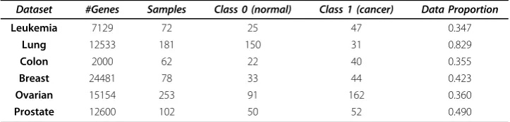
In this section, six free-public cancer datasets (http://datam.i2r.a-star.edu.sg/datasets/ krbd/index.html) have been used to test the proposed methodology. The main charac-teristics (# genes, # samples, and class distribution) for each dataset is shown in Table 1. A comparison between the two analyzed frameworks is conducted, where for each meth-odology six classification techniques are applied, namely: LDA, SVM, NaiveBayes, C-MANTEC, kNN and MLP.

Before applying the methodology based on genetic algorithms, it is necessary to esti-mate the parameters aandbassociated with the fitness function and referred in a pre-vious section. This estimation is carry out for all the cancer datasets, although only the information related to theLungand P rostatedatasets are shown by the sake of simpli-city. Different combinations of the land b parameters together with the accuracy results on average and number of selected genes are shown in Table 2. The differences in the accuracy rates for each parameter combination are not statistically significant, which implies that, for these cancer datasets, any combination of parameters can be chosen. Specifically, the combinationsa = 0.4,b= 0.25 anda= 0.1,b= 0.25 (Table 2, in italic), lead to the obtention of the largest success rate, taking into account that when a is reduced (a = 0.1) the number of genes in the solution is a little higher (12.78 in P rostateand 4.73 inLung) than when we try to minimise the solution with more emphasis (a= 0.4, 9.32 genes inP rostateand 4.25 inLung, on average).

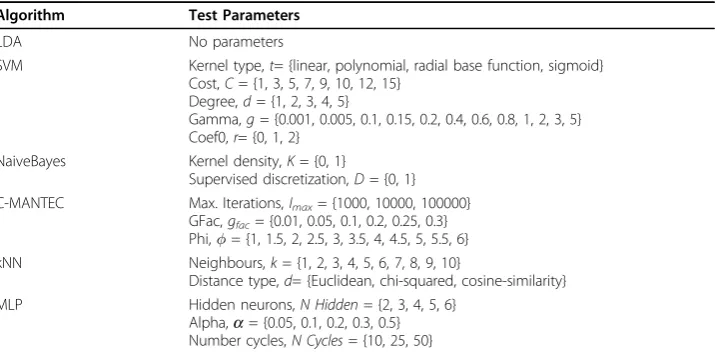
Table 3 shows the set of parameters that have to be set for each classifier, together with the different values that have been tested in this paper. For each classifier, a hold-out validation strategy is used by dividing the entire dataset on a 60 −40% proportion; the first set to train the model and the second to obtain the accuracy in the prediction of cancer outcome. The training-testing procedure is repeated 50 times randomly vary-ing the trainvary-ing and testvary-ing set to avoid a biased evaluation, permittvary-ing also to analyse the dispersion of the results.

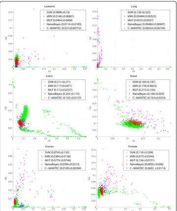
A thorough analysis of the parameter setting is presented in Figure 1, where its influ-ence for the different algorithms is evaluated in the variability of the classification

Table 1 Cancer datasets

Dataset #Genes Samples Class 0 (normal) Class 1 (cancer) Data Proportion

Leukemia 7129 72 25 47 0.347

Lung 12533 181 150 31 0.829

Colon 2000 62 22 40 0.355

Breast 24481 78 33 44 0.423

Ovarian 15154 253 91 162 0.360

Prostate 12600 102 50 52 0.490

accuracy. The horizontal axis corresponds to the average percentage across the 50 samples considered of the false positives (FP) of the data, while the vertical axis is associated with the false negatives values (FN). Each point of the plot represents the

FPand FNvalues of a generated configuration with a given parameter setting. The clo-ser the points are to the origin, the better the classification accuracy, with optimum performance occurring forFN =FP= 0 (a perfect match between the output of the algorithm and the observed outcome of the dataset). All points are located always below the contradiagonal of the plot (FN+FP= 1) as it is verified thatFN +FP≤1.

The variability observed for each classifier depends largely on the analysed dataset, but with the robustness of each of the method having also a strong influence, as more robust methods yield to more compact configuration clouds of points (a compact con-figuration cloud means that the results do not vary significantly after a change in the classifier parameters). Thus, the compactness can be defined as the standard deviation of the accuracy measures. As shown in Figure 1, the compactness for kNN, SVM and MLP methods is rather poor in general, while the C-MANTEC approach leads to con-figurations that are very close together, indicating clearly that the performance of this method is not very sensitive to the parameter selection. Additionally, C-MANTEC lead to the lowest values for the distance of the mean of the configuration values (FP and

Table 2 Parameters estimation for GA

Prostate dataset Lung dataset

a b Accuracy #Genes a b Accuracy #Genes

0.8 0.6 0.9838±0.0097 2.67±1.19 0.8 0.6 0.9730±0.0107 8.65±2.82

0.8 0.4 0.9899±0.0072 3.30±1.02 0.8 0.4 0.9748±0.0093 7.28±1.20

0.8 0.25 0.9914±0.0054 3.52±0.91 0.8 0.25 0.9801±0.0106 9.85±3.12

0.4 0.6 0.9827±0.0086 2.56±1.01 0.4 0.6 0.9743±0.0103 8.80±3.18

0.4 0.4 0.9912±0.0069 3.75±1.44 0.4 0.4 0.9763±0.0094 9.55±1.08

0.4 0.25 0.9938 ± 0.0061 4.25 ± 1.95 0.4 0.25 0.9849 ± 0.0089 9.32 ± 1.64

0.1 0.6 0.9837 ± 0.0104 3.04 ± 1.71 0.1 0.6 0.9770 ± 0.0095 7.83 ± 2.06

0.1 0.4 0.9895 ± 0.0065 2.88 ± 0.70 0.1 0.4 0.9763 ± 0.0118 9.63 ± 2.53

0.1 0.25 0.9966 ± 0.0041 4.73 ± 2.10 0.1 0.25 0.9854 ± 0.0101 12.78 ± 1.61

Parameter estimation for theaandbparameters of the fitness function of the GA for theLungandProstatedatasets.

Table 3 Parameters settings

Algorithm Test Parameters

LDA No parameters

SVM Kernel type,t= {linear, polynomial, radial base function, sigmoid} Cost,C= {1, 3, 5, 7, 9, 10, 12, 15}

Degree,d= {1, 2, 3, 4, 5}

Gamma,g= {0.001, 0.005, 0.1, 0.15, 0.2, 0.4, 0.6, 0.8, 1, 2, 3, 5} Coef0,r= {0, 1, 2}

NaiveBayes Kernel density,K= {0, 1}

Supervised discretization,D= {0, 1} C-MANTEC Max. Iterations,Imax= {1000, 10000, 100000}

GFac,gfac= {0.01, 0.05, 0.1, 0.2, 0.25, 0.3}

Phi,= {1, 1.5, 2, 2.5, 3, 3.5, 4, 4.5, 5, 5.5, 6}

kNN Neighbours,k= {1, 2, 3, 4, 5, 6, 7, 8, 9, 10}

Distance type,d= {Euclidean, chi-squared, cosine-similarity}

MLP Hidden neurons,N Hidden= {2, 3, 4, 5, 6}

Alpha,a= {0.05, 0.1, 0.2, 0.3, 0.5} Number cycles,N Cycles= {10, 25, 50}

FN) to the origin, confirming the robustness in the parameter setting (the LDA classi-fier does not have parameters to be set and thus it is not represented in the graph). In order to quantify the distribution of the prediction accuracy observed for the several configuration analysed, the legend for each classifier shows the distance to the plot

ori-gin plus/minus the standard deviation

(FP)2+ (FN)2±std-dev

. For example, for

the Ovarian, ColonandProstate datasets, the distance to the origin for the mean value observed for the C-MANTEC algorithm is significantly lower than for the rest of alter-natives (0.0109, 0.102 and 0.0602, respectively).

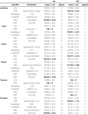
Comparison results between the two frameworks are shown in Table 4, where the best parameter configuration for each classification model is selected to perform the evalua-tion over the six datasets. In both frameworks, the accuracy rates for theLeukemia,

LungandOvariandatasets are close to 100% regardless of the classifier applied, suggest-ing a low data complexity (in prediction terms). The complexity theBreast, Colonand

Prostate seems higher, permitting to observe clear differences between the two approaches. The prediction accuracy obtained with the GA methodology was in almost all cases higher that the obtained within the SFS approach. Additionally, the robustness of the selected features is considerably higher in the GA (lower standard deviation

Table 4 Performance comparison of classification techniques

GA SFS

Classifier Parameters mean ± std #genes mean ± std #genes

Leukemia LDA - 99.959 ± 0.07 12 97.609 ± 2.86 2

SVM {polynomial,15,1,0.6,0} 99.982 ± 0.06 8 99.918 ± 0.52 4

NaiveBayes {1,0} 99.974 ± 0.03 12 98.060 ± 2.19 3

C-MANTEC {1000,0.01,4.5} 99.038 ± 0.25 7 98.837 ± 2.46 3

kNN {1,Euclidean} 99.994 ± 0.02 10 99.844 ± 0.77 5

MLP {3,0.5,50} 99.944 ± 0.05 5 95.784 ± 3.38 2

Lung LDA - 99.971 ± 0.03 5 99.057 ± 1.00 3

SVM {linear,10,-,-,-} 100 ± 0 11 99.828 ± 0.70 3

NaiveBayes {1,0} 99.998 ± 0.01 4 99.991 ± 0.07 3

C-MANTEC {100000,0.25,2} 99.678 ± 0.08 6 99.673 ± 0.94 2

kNN {1,Euclidean} 99.969 ± 0.02 4 99.969 ± 0.22 4

MLP {4,0.1,50} 99.996 ± 0.01 4 99.778 ± 0.79 2

Colon LDA - 98.676 ± 0.35 11 87.179 ± 6.15 2

SVM {polynomial,1,1,0.4,2} 89.917 ± 1.26 20 91.738 ± 5.21 5

NaiveBayes {0,1} 90.583 ± 0.49 15 89.076 ± 7.79 4

C-MANTEC {10000,0.01,1} 94.315 ± 0.48 11 87.593 ± 6.69 2

kNN {3,cosine-similarity} 95.060 ± 0.38 19 93.577 ± 4.43 6

MLP {5,0.3,50} 99.026 ± 0.30 12 88.733 ± 5.51 2

Breast LDA - 99.788 ± 0.12 15 74.169 ± 6.52 1

SVM {polynomial,7,2,0.001,2} 99.744 ± 0.14 31 81.029 ± 5.80 3

NaiveBayes {0,0} 97.759 ± 0.23 27 73.499 ± 6.34 1

C-MANTEC {10000,0.01,1.5} 97.342 ± 0.39 23 76.645 ± 6.53 1

kNN {3,Euclidean} 97.485 ± 0.30 34 80.975 ± 6.37 2

MLP {4,0.3,50} 99.828 ± 0.09 18 79.191 ± 6.43 2

Ovarian LDA - 99.980 ± 0.01 4 100 ± 0 3

SVM {polynomial,9,1,0.2,0} 100 ± 0 4 99.978 ± 0.13 4

NaiveBayes {1,0} 99.951 ± 0.03 5 99.980 ± 0.13 4

C-MANTEC {1000,0.3,1.5} 99.844 ± 0.05 4 99.659 ± 0.75 3

kNN {1,Euclidean} 99.984 ± 0.01 4 99.982 ± 0.11 3

MLP {5,0.3,50} 99.999 ± 0 3 100 ± 0 3

Prostate LDA - 99.720 ± 0.12 9 95.677 ± 2.81 4

SVM {polynomial,5,1,3,1} 99.428 ± 0.31 20 98.622 ± 1.79 5

NaiveBayes {0,0} 98.817 ± 0.16 14 98.331 ± 2.13 7

C-MANTEC {1000,0.25,4} 98.681 ± 0.24 8 95.351 ± 3.40 4

kNN {3,cosine-similarity} 99.633 ± 0.11 20 97.146 ± 2.28 6

MLP {3,0.5,50} 99.996 ± 0.02 12 96.921 ± 2.37 4

Performance comparison among the two different feature selection frameworks used (GA and SFS) and the six classifiers analyzed (LDA, SVM, NaiveBayes, C-MANTEC, kNN and MLP) for each cancer microarray dataset. The results correspond to the best simulation for each dataset, showing the accuracy for method in the format ofmean ± standard deviation

values), fact that can be partially attributed to the larger set of genes selected. Regarding the computational complexity of both approaches, the SFS strategy involves approxi-mately a number of comparisons of nsel×#genes (nsel: number of pre-selected features, #genes: mean number of genes selected), while the GA approach utilises a maximum of 20.000 profile comparisons regardless of the dataset (length of the chromosome (100)× number of generations (200)). For example, for theProstatedataset in the SFS approach, approximately 3000 comparison are needed in the present study since nsel≈600, #genes= 5, unlike the genetic proposal which requires a greater number of combina-tions. However, if the number of pre-selected genes increases, the SFS method begins to loose its efficiency and may be intractable when handling thousands of genes.

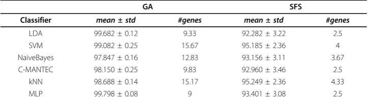
Table 5 shows average results across all six datasets for the both frameworks used, noting that C-MANTEC lead to competitive classification performance with a reduced number of genes.

Further, we analyzed the differences between classifiers for the SFS and GA feature selection procedures used and for the six datasets, showing the results in Table 6. The corresponding p-value obtained after applying a Friedman’s test is indicated in the third column [28]. In case this p-value is lower than 0.05, the lowest performant classi-fier is taken as a control group and the last column of the table lists the classiclassi-fiers that lead to statistically significant results (from the lowest to the highest difference);

Table 5 Performance comparison of feature selection frameworks

GA SFS

Classifier mean ± std #genes mean ± std #genes

LDA 99.682 ± 0.12 9.33 92.282 ± 3.22 2.5

SVM 99.082 ± 0.25 15.67 95.185 ± 2.36 4

NaiveBayes 97.847 ± 0.16 12.83 93.156 ± 3.11 3.67

C-MANTEC 98.150 ± 0.25 9.83 92.960 ± 3.46 2.5

kNN 98.688 ± 0.14 15.17 95.249 ± 2.36 4.33

MLP 99.798 ± 0.08 9 93.401 ± 3.08 2.5

Average performance comparison among two different feature selection frameworks (GA and SFS) and six classifiers (LDA, SVM, NaiveBayes, C-MANTEC, kNN and MLP) over all dataset.

Table 6 Differences between classifiers.

FS procedure Dataset p-value Control Statistically different classifiers

SFS Leukemia < e−16 LDA SVM

Lung < e−16 LDA kNN, NB

Colon < e−16 LDA SVM, kNN

Breast < e−16 NB kNN, SVM

Ovarian < e−16 _{CM LDA, NN}

Prostate < e−16 _{CM NB, SVM}

GA Leukemia < e−16 _{CM NB, NN, LDA, SVM, kNN}

Lung < e−16 _{CM SVM, NB, NN}

Colon < e−16 _{SVM LDA, NN}

Breast < e−16 _{SVM NN, LDA}

Ovarian < e−16 _{CM SVM, NN}

Prostate < e−16 CM NN, LDA

otherwise, non statistically significant results are reached (represented with a “-” on the table).

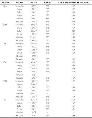
Table 7 shows a similar comparative analysis but among the SFS and GA feature selection procedures when a common classifier is used (first column of the table).

Biological analysis

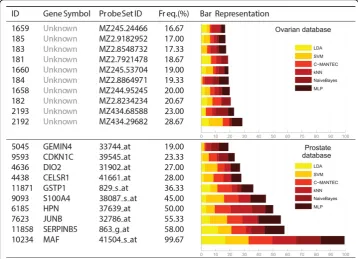
Figures 2 and 3 present the ten most selected genes for each of the six datasets consid-ered, where each dataset is represented in a row of the table. The first three columns show information about the gene, such as the internal index (ID), the gene symbol (name of the gene) and the probe set ID, which is related to the chip where the dataset

Table 7 Differences between feature selection algorithms

Classifier Dataset p-value Control Statistically different FS procedures

LDA Leukemia 1.54e−12 SFS GA

Lung 1.54e−12 SFS GA

Colon 1.54e−12 _{SFS GA}

Breast 1.54e−12 _{SFS GA}

Ovarian 3.28e−11 _{GA SFS}

Prostate 1.54e−12 _{SFS GA}

SVM Leukemia 3.65e−5 _{SFS GA}

Lung 1.54e−12 _{SFS GA}

Colon 2.86e−9 _{GA SFS}

Breast 1.54e−12 _{SFS GA}

Ovarian 9.13e−11 SFS GA

Prostate 1.54e−12 SFS GA

NB Leukemia 4.71e−9 SFS GA

Lung 1.54e−12 SFS GA

Colon 1.54e−12 SFS GA

Breast 1.54e−12 SFS GA

Ovarian 0.157 -

-Prostate 1.54e−12 SFS GA

CM Leukemia 4.71e−9 _{SFS GA}

Lung 1.54e−12 _{SFS GA}

Colon 1.54e−12 _{SFS GA}

Breast 1.54e−12 _{SFS GA}

Ovarian 0.157 -

-Prostate 1.54e−12 _{SFS GA}

kNN Leukemia 1.54e−12 SFS GA

Lung 0.0897 -

-Colon 1.54e−12 SFS GA

Breast 1.54e−12 SFS GA

Ovarian 0.6547 -

-Prostate 1.54e−12 SFS GA

NN Leukemia 4.71e−9 SFS GA

Lung 1.54e−12 SFS GA

Colon 1.54e−12 _{SFS GA}

Breast 1.54e−12 _{SFS GA}

Ovarian 0.157 -

-Prostate 1.54e−12 _{SFS GA}

has been extracted (e.g., Affymetrix). The bar graph of the last column splits the fre-quency of selection (fourth column) of each feature according to the LDA, GA-SVM, GA-CMANTEC, GA-kNN, GA-NaiveBayes and GA-MLP strategies. Most of the gene symbols have been found from their probe set ID by using tools as IPA (Ingenuity®

Figure 2Frequency selection of genes for Leukemia, Lung, Colon and Breast databases. The ten most selected features for the analysed datasets. Frequency selection is represented by an horizontal bar, divided according to the six classifiers used in the analysis: LDA, SVM, C-MANTEC, kNN, NaiveBayes and MLP. The index, gene symbol and probe set ID of each gene is shown in columns one to three.

Systems, http://www.ingenuity.com) or NCBI (http://www.ncbi.nlm.nih.gov/gene/), although it has not been possible for theOvariandataset (first row of Figure 3) because there is no reference of the chip from which the data have been extracted.

A higher frequency of selection might imply a higher relevance of the gene in the prognosis of the disease. Those genes that are selected with similar frequency for all classifiers are considered independent with respect to the classification method. For instance, in the Prostatedataset (second row of Figure 3), the MAF gene is more sig-nificant than the JUNB gene, since it has been selected more times and all the classi-fiers selects it with the same frequency. Thus, NaiveBayesbarely takes into account the JUNB gene whereas for MLP classifier it is one of the main genes.

Not only are we interested in getting good results in prognosis prediction but also in examining whether the selected genes provide biological information related to the dis-ease studied. Therefore, if the proposed models provide this consistency between the computational and biological field, the results would be more confident and the selected genes would be more reliable from a clinical perspective, in order to their implementation in microchips and treatment in real patients. We can see that this statement is true in the proposed model using genetic algorithms.

In the case of theProstatedataset is possible to find references in the literature where the genesMAF, which encodes a protein related to DNA-binding (most frequent gene, 99.67%) [29],SERPINB5, a serpin peptidase inhibitor (second most frequent, 58%) [30], HPN, officially named hepsin which encodes a type II transmembrane serine protease (fourth most frequent, 50%) [31] andGSTP1, belonging to the family of Glutathione S-transferases (GSTs) enzymes (sixth most frequent, 36.33%) [32] are biologically related to the absence or presence of prostate cancer. This supports the idea that our computa-tional approach is robust and consistent with the results obtained in biological studies.

For the Breast dataset, several of the most selected genes among which areUBC [33,34], ZNF222[35] andEWSR1[36], are biologically associated with breast cancer. The same happen for the Leukemiadisease, where the enforced expression of the CD19 molecule (fifth selected, 19%) can reduce the proliferation of the malignant plasma cells [37]; the gene homeobox A9 (HOXA9, second selected, 33%) influences hematopoietic progenitors and acute leukemias [38]; and the CD33molecule (seventh selected, 17.33%) has been shown to sharply inhibit the in vitro proliferation of both normal myeloid cells and chronic myeloid leukemias [39].

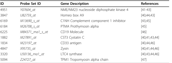
From a computational point of view, Table 8 shows the best selected genes obtained by the genetic approach which also have been extracted in several related papers (last column of the table) for the particular case of the Leukemia dataset. It should be noted that the applied methodology is different from one paper to another. For instance, five of the ten genes are also reported in the list of the 50 most important genes (selected from 7129) suggested in [40].

founded genes in the IPA database with biological relevance on the Leukemia cancer disease.

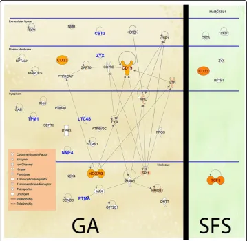
A deeper biological analysis is performed using the IPA tool for the GA-CMANTEC strategy considering theLeukemiadataset. Figure 5 shows those genes that are selected at least a 5% of the times both with GA-CMANTEC or SFS-CMANTEC strategy after 50 independent executions. The names shown on this figure correspond to the symbol of each gene according to Figure 2. It is important to highlight the difference on the number of genes selected through the GA and SFS strategy due to the casuistic of each algorithm. Additionally, on the left side are represented in bold nine of the ten most frequently selected genes with independence of the classifier used. Moreover, using C-MANTEC as classifier allow to obtain these nine most selected genes. Finally, filled in genes represent those genes that have demonstrate biological relevance on the Leukemia disease. In this sense, the GA-CMANTEC strategy presents 10 out of 37 genes as a result while the SFS-CMANTEC strategy presents 2 out of 7. Although these results are similar in proportion, the GA-CMANTEC strategy could be consid-ered more explicative from a biological point view with no detriment on the classifica-tion performance. Furthermore, the connecclassifica-tions among the selected genes (represented by links in Figure 5), which are more numerous in the GA approach, sug-gest as well a significant relationship with the occurrence of the disease.

Conclusions

In this work, a new methodology approach combining genetic algorithm with con-structive neural networks has been proposed in order to predict cancer outcome. For six free-public cancer datasets, we compared under GA and SFS frameworks the pre-diction accuracy of the C-MANTEC algorithm against the following five standard clas-sifiers: LDA, SVM, NaiveBayes, kNN or MLP.

On average, the strategy based on the GA approach leads to better prediction rates, observing that these results are independent of the classifier used, noting also that pre-diction results under the GA framework show lower variability, and thus can be con-sidered as more robust. On the other hand, it should be noted that the SFS approach is less computationally intensive, involving in the present study approximately seven times less gene comparisons, and also leading to a group of selected genes much smal-ler than those selected under the GA approach. Nevertheless, when complex datasets

Table 8 Selected genes for the Leukemia dataset

ID Probe Set ID Gene Description References

4951 Y07604_at NME/NM23 nucleoside diphosphate kinase 4 [41-43]

3847 U82759_at Homeo box A9 [40,44,43]

6169 M13690_s_at C1NH Complement component 1 inhibitor [43,45]

6184 M26708_s_at PTMA Prothymosin alpha [45]

6225 M84371_rna1_s_at CD19 Molecule [46]

1882 M27891_at CST3 Cystatin C [40,41,43,44]

1834 M23197_at CD33 antigen [40,44,46]

4847 X95735_at Zyxin [40,41,44,46]

3320 U50136_rna1_at LTC4 synthase [40,43,44,46]

5094 Z24727_at TPM1 Tropomyosin alpha chain [47]

are studied like Breastor Colon, cancer prognosis results are quite poor when using the SFS approach, presumably since the search in the state space is much more restric-tive. Additionally, an analysis done using the IPA methodology suggests that the biolo-gical relevance of the genes selected under the GA framework is higher than the observed using the SFS approach, as indicated by the reference frequency in the litera-ture and also regarding the relationship between them (even if this effect might be due to the size of both selected sets).

Regarding the comparison between the different classifiers implemented, standard feed-forward neural networks (MLP), LDA and SVM lead to similar and best results while C-MANTEC and kNN followed closely but with a bit lower accuracy. C-MANTEC, MLP and LDA permitted to obtain a more reduced set of genes in comparison to SVM, NB and kNN. Further, C-MANTEC resulted in the most robust classifier in terms of changes in the parameter settings, a relevant feature for its use in wrapper feature selection methods (as it will reduce execution times related to parameter tuning). Additionally, we are con-sidering the use of a ensemble of all these classifiers as a further work, in order to obtain a greater consensus on the classification result, which could lead to greater robustness and accuracy of the resulting model.

Competing interests

The authors declare that they have no competing interests.

Authors_’contributions

RML, DU and JMJ contributed to the conception and design of the study. RML, DU and JLS contributed to write the programming code. RML, DU, JMJ and LF contributed to the analysis and interpretation of the data, and RML, DU, LF and JMJ contributed to the drafting of the manuscript. All authors approved the manuscript.

Declarations

Publication funding for this article has come from grants TIN2010-16556 (MICINN-Spain) and TIC-4026/2008 (Consejería de Innovación, Ciencia y Empresa. Junta de Andalucía), both including FEDER funds. Additionally, the authors acknowledge support through these grants.

This article has been published as part ofTheoretical Biology and Medical ModellingVolume 11 Supplement 1, 2014: Selected articles from the 1st International Work-Conference on Bioinformatics and Biomedical Engineering-IWBBIO 2013. The full contents of the supplement are available online at http://www.tbiomed.com/supplements/11/S1.

Authors_’details 1

Department of Computer Science, University of Málaga, Málaga, Spain.2Biomedical Research Institute of Málaga (IBIMA), Spain.

Published: 7 May 2014

References

1. Wei JS, Greer BT, Westermann F, Steinberg SM, Son CG:Prediction of Clinical Outcome Using Gene Ex-pression Profiling and Artificial Neural Networks for Patients with Neuroblastom.Cancer Research2004,64:6883-6891. 2. Pellagatti A, Vetrie D, Langford CF, Gama S, Eagleton H, Wainscoat JS, Boultwood J:Gene Expression Profiling in

Polycythemia Vera Using cDNA Microarray Technology.Cancer Research2003,63:3940-3944. 3. West M:Bayesian factor regression models in the_“large p, small n_”paradigm.Bayesian statistics2003,

7(2003):723-732.

4. Ransohoff D:Rules of evidence for cancer molecular-marker discovery and validation.Nature Reviews Cancer2004,

4(4):309-314.

5. Lancashire LJ, Rees RC, Ball GR:Identification of gene transcript signatures predictive for estrogen receptor and lymph node status using a stepwise forward selection artificial neural network modelling approach.Artificial Intelligence In Medicine2008,43(2):99-111.

6. Peng H, Fu Y, Liu J, Fang X, Jiang C:Optimal gene subset selection using the modified SFFS algorithm for tumor classification.Neural Computing and Applications2012, 1-8.

7. Raymer M, Punch W, Goodman E, Kuhn L, Jain A:Dimensionality reduction using genetic algorithms.IEEE Transactions on Evolutionary Computation2000,4(2):164-171.

8. Chiang Y, Chiang H, Lin S:The application of ant colony optimization for gene selection in microarray-based cancer classification.Proceedings of the 7th International Conference on Machine Learning and Cybernetics, ICMLC2008,

7:4001-4006.

9. Sun Z, Bebis G, Miller R:Object detection using feature subset selection.Pattern Recognition2004,37(11):2165-2176. 10. McLachlan G, Bean R, Peel D:A mixture model-based approach to the clustering of microarray expression data.

Bioinformatics2002,18(3):413-422.

11. Molinaro A, Simon R, Pfeiffer R:Prediction error estimation: a comparison of resampling methods.Bioinformatics

2005,21(15):3301-3307.

12. Zhang F, Kaufman HL, Deng Y, Drabier R:Recursive SVM biomarker selection for early detection of breast cancer in peripheral blood.BMC Medical Genomics2013,6(1).

13. Tong DL, Schierz AC:Hybrid genetic algorithm-neural network: Feature extraction for unpreprocessed microarray data.Artificial Intelligence in Medicine2011,53:47-56.

14. Su Y, Wang R, Li C, Chen P:A dynamic subspace learning method for tumor classification using microarray gene expression data.Proceedings - 2011 7th International Conference on Natural Computation, ICNC 20112011,1:396-400. 15. Student S, Fujarewicz K:Stable feature selection and classification algorithms for multiclass microarray data.Biology

Direct2012,7.

16. Werner T:Bioinformatics applications for pathway analysis of microarray data.Current Opinion in Biotechnology2008,

19:50-54.

17. Subirats JL, Franco L, Jerez JM:C-Mantec: A novel constructive neural network algorithm incorporating competition between neurons.Neural Networks2012,26:130-140.

18. Saeys Y, Inza I, Larranãga P:A review of feature selection techniques in bioinformatics.Bioinformatics2007,

23(19):2507-2517.

19. Huerta EB, Duval B, Hao JK:A hybrid LDA and genetic algorithm for gene selection and classification of microarray data.Neurocomputing2010,73:2375-2383.

20. Welch BL:The generalization of Student´s problem when several different population variances are involved.

Biometrika1947,34(1-2):28-35.

21. Webb AR:Statistical Pattern Recognition.2 edition. John Wiley & Sons; 2011, third edition.

22. Peng H, Long F, Ding C:Feature selection based on mutual information criteria of dependency, max-relevance, and min-redundancy.IEEE Transactions on Pattern Analysis and Machine Intelligence2005,27(8):1226-1238. 23. Guo B, Nixon M:Gait Feature Subset Selection by Mutual Information.IEEE Transactions on Systems, Man and

Cybernetics, Part A: Systems and Humans2009,39:36-46.

24. Moddemeijer R:On Estimation of Entropy and Mutual Information of Continuous Distributions.Signal Processing

1989,16(3):233-246.

25. Frean M:A_“thermal_”perceptron learning rule.Neural Comput.1992,4(6):946-957.

26. García-Pedrajas N, Ortiz-Boyer D:A cooperative constructive method for neural networks for pattern recognition.

Pattern Recogn.2007,40:80-98.

27. Subirats JL, Jerez JM, Franco L:A New Decomposition Algorithm for Threshold Synthesis and Generalization of Boolean Functions.IEEE Transactions on Circuits and Systems2008,1(55):3188-3196.

28. García S, Fernández A, Luengo J, Herrera F:Advanced nonparametric tests for multiple comparisons in the design of experiments in computational intelligence and data mining: Experimental analysis of power.Information Sciences

2010,180(10):2044-2064.

29. Steele VE, Arnold JT, Le H, Izmirlian G, Blackman MR:Comparative Effects of DHEA and DHT on Gene Expression in Human LNCaP Prostate Cancer Cells.Anticancer Research2006,26(5A):3205-3215.

30. Sheng S, Carey J, Seftor EA, Dias L, Hendrix MJ, Sager R:Maspin acts at the cell membrane to inhibit invasion and motility of mammary and prostatic cancer cells.Proc Natl Acad Sci USA1996,93(21):11669-74.

31. Srikantan V, Valladares M, Rhim JS, Moul JW, Srivastava S:HEPSIN Inhibits Cell Growth/Invasion in Prostate Cancer Cells.Cancer Research2002,62(23):6812-6816.

32. Lin X, Tascilar M, Lee WH, Vles WJ, Lee BH, Veeraswamy R, Asgari K, Freije D, van Rees B, Gage WR, Bova GS, Isaacs WB, Brooks JD, DeWeese TL, Marzo AMD, Nelson WG:{GSTP1} CpG Island Hypermethylation Is Responsible for the Absence of {GSTP1} Expression in Human Prostate Cancer Cells.The American Journal of Pathology2001,

33. Ramachandran C, Rodriguez S, Ramachandran R, Nair PR, Fonseca H, Khatib Z, Escalon E, Melnick SJ:Expression Profiles of Apoptotic Genes Induced by Curcumin in Human Breast Cancer and Mammary Epithelial Cell Lines.Anticancer Research2005,25(5):3293-3302.

34. Kroll T, Odyvanova L, Clement J, Platzer C, Naumann A, Marr N, Höffken K, Wölfl S:Molecular characterization of breast cancer cell lines by expression profiling.Journal of Cancer Research and Clinical Oncology2002,128(3):125-134. 35. Klein A, Olendrowitz C, Schmutzler R, Hampl J, Schlag PM, Maass N, Arnold N, Wessel R, Ramser J, Meindl A,

Scherneck S, Seitz S:Identification of brain-and bone-specific breast cancer metastasis genes.Cancer Letters2009,

276(2):212-220.

36. Menon R, Omenn GS:Proteomic Characterization of Novel Alternative Splice Variant Proteins in Human Epidermal Growth Factor Receptor 2 neu Induced Breast Cancers.Cancer Research2010,70(9):3440-3449.

37. Mahmoud MS, Fujii R, Ishikawa H, Kawano MM:Enforced CD19 Expression Leads to Growth Inhibition and Reduced Tumorigenicity.Blood1999,94(10):3551-3558.

38. Hu YL, Fong S, Ferrell C, Largman C, Shen WF:HOXA9 Modulates Its Oncogenic Partner Meis1 To Influence Normal Hematopoiesis.Molecular and Cellular Biology2009,29(18):5181-5192.

39. Vitale C, Romagnani C, Puccetti A, Olive D, Costello R, Chiossone L, Pitto A, Bacigalupo A, Moretta L, Mingari MC:

Surface expression and function of p75/AIRM-1 or CD33 in acute myeloid leukemias: Engagement of CD33 induces apoptosis of leukemic cells.Proceedings of the National Academy of Sciences2001,98(10):5764-5769. 40. Golub T, Slonim D, Tamayo P, Huard C, Gaasenbeek M, Mesirov J, Coller H, Loh M, Downing J, Caligiuri M, Bloomfield C,

Lander E:Molecular classification of cancer: Class discovery and class prediction by gene expression monitoring.

Science1999,286(5439):531-537.

41. Yang P, Zhou BB, Zhang Z, Zomaya AY:A multi-filter enhanced genetic ensemble system for gene selection and sample classification of microarray data.BMC Bioinformatics2010,11(1).

42. García-Nieto J, Alba E, Jourdan L, Talbi E:Sensitivity and specificity based multiobjective approach for feature selection: Application to cancer diagnosis.Information Processing Letters2009,109(16):887-896.

43. Krishnapuram B, Carin L, Hartemink A:Joint classifier and feature optimization for comprehensive cancer diagnosis using gene expression data.Journal of Computational Biology2004,11(2-3):227-242.

44. Chen Z, Li J, Wei L:A multiple kernel support vector machine scheme for feature selection and rule extraction from gene expression data of cancer tissue.Artificial Intelligence in Medicine2007,41(2):161-175.

45. Shen Q, Shi WM, Kong W:Hybrid particle swarm optimization and tabu search approach for selecting genes for tumor classification using gene expression data.Computational Biology and Chemistry2008,32:53-60.

46. Momin B, Mitra S, Gupta R:Reduct Generation and Classification of Gene Expression Data.Hybrid Information Technology, 2006 ICHIT‘06 International Conference on2006,1:699-708.

47. Gwinn M, Keshava C, Olivero O, Humsi J, Poirier M, Weston A:Transcriptional signatures of normal human mammary epithelial cells in response to benzo[a]pyrene exposure: a comparison of three microarray platforms.OMICS2005,

9(4):334-50.

doi:10.1186/1742-4682-11-S1-S7

Cite this article as:Luque-Baenaet al.:Application of genetic algorithms and constructive neural networks for the analysis of microarray cancer data.Theoretical Biology and Medical Modelling201411(Suppl 1):S7.

Submit your next manuscript to BioMed Central and take full advantage of:

• Convenient online submission

• Thorough peer review

• No space constraints or color figure charges

• Immediate publication on acceptance

• Inclusion in PubMed, CAS, Scopus and Google Scholar

• Research which is freely available for redistribution