Sentiment classification with deep neural networks

(1)

SENTIMENT CLASSIFICATION WITH DEEP

NEURAL NETWORKS

Faculty of Information Technology and Communication Sciences Master of Science thesis May 2019

(2)

ABSTRACT

Yi Zhou: Sentiment classification with deep neural networks Master of Science thesis

Tampere University

Master’s Degree Programme in Software Development May 2019

Sentiment classification is an important task in Natural Language Processing (NLP) area. Deep neural networks become the mainstream method to perform the text sentiment classifica-tion nowadays. In this thesis two datasets are used. The first dataset is a hotel review dataset (TripAdvisor dataset) that collects the hotel reviews from the TripAdvisor website using Python Scrapy framework. The pre-processing steps are then applied to clean the dataset. A record in the TripAdvisor dataset consists of the text review and corresponding sentiment score. There are 5 sentimental labels: very negative, negative, neutral, positive, and very positive. The second dataset is the Stanford Sentiment Treebank (SST) dataset. It is a public and common dataset for sentiment classification.

Text Convolutional Neural Network (Text-CNN), Very Deep Convolutional Neural Network (VD-CNN), and Bidirectional Long Short Term Memory neural network (BiLSTM) were chosen as different methods for the evaluation in the experiments. The Text-CNN was the first work to apply convolutional neural network architecture for the text classification. The VD-CNN applied deep convolutional layers, with up to 29 layers, to perform the text classification. The BiLSTM exploited the bidirectional recurrent neural network with long short term memory cell mechanism. On the other hand, word embedding techniques are also considered as an important factor in sentiment classification. Thus, in this thesis, GloVe and FastText techniques were used to investigate the effect of word embedding initialization on the dataset. GloVe is a unsupervised word embedding learning algorithm. FastText uses shallow neural network to generate word vectors and it has fast convergence speed for training and high speed for inference.

The experiment was implemented using PyTorch framework. It shows that the BiLSTM with GloVe as the word vector initialization achieved the highest accuracy 73.73% while the VD-CNN with FastText had the lowest accuracy 71.95% on the TripAdvisor dataset. The BiLSTM model achieved 0.68 F1-score while the VD-CNN model obtained 0.67 F1-score on the TripAdvisor dataset. On the SST dataset, BiLSTM with GloVe again achieved the highest accuracy 36.35% and 0.35 F1-score. The VD-CNN model with GloVe had the worst evaluation result in terms of accuracy and F1-score. The Text-CNN model performed better than the VD-CNN model even thought the VD-CNN model has more layers in most cases.

By analyzing the misclassified reviews in the TripAdvisor dataset from the three deep neural networks, it is shown that the hotel reviews with more contradictory sentimental words were more prone to misclassification than other hotel reviews.

Keywords: deep neural networks, convolutional neural network, recurrent neural network, senti-ment classification, hotel reviews, TripAdvisor

(3)

PREFACE

I want to express my deep gratitude to my supervisors, Prof. Jyrki Nummenmaa, Asso-ciate Prof. Kostas Stefanidis and AssoAsso-ciate Prof. Heikki Huttunen. They introduced me into this research area. Without their guide, this master thesis is not possible to complete. Apart from the supervision, I would like to appreciate the kindness and patience of my supervisors since the thesis took a long time to complete.

I would like to express my thanks to my family. They help me a lot for my study in this lovely country, Finland. I also express my thanks for my colleges, they provided lots of help during the process of writing the thesis.

Tampere, Finland, 20th May 2019 Yi Zhou

(4)

LIST OF FIGURES

2.1 The structure of a single neuron . . . 4

2.2 Sigmoid and Tanh activation function . . . 4

2.3 ReLU and leaky ReLU activation function . . . 5

2.4 Typical architecture of the multi-layer perceptron . . . 6

2.5 Convolution operation illustration . . . 6

2.6 Max pooling and average pooling operation comparison . . . 7

2.7 Four types of RNN models . . . 9

2.8 The unfolding recurrent neural network along with time steps [9] . . . 10

2.9 LSTM cell structure [56] . . . 11

2.10 The structure of the bidirectional recurrent neural network . . . 12

2.11 Stochastic gradient descent optimization algorithm for the functionf(x) = x2 1+ 2x22[56] . . . 13

2.12 Overfitting in deep neural networks [9] . . . 14

2.13 The structure comparison of MLP with and without dropout technique . . . 15

2.14 Overview of word embedding technique . . . 18

2.15 The continuous-bag-of-words versus the skipgram method [14] . . . 19

2.16 Two-dimensional principal component analysis projection of the word vec-tors of countries and corresponding capital cities [35] . . . 20

2.17 FastText model architecture for generating the vector representation for a sentence with ngram featuresx1, . . . ,xN [19] . . . 20

3.1 A original hotel review on the TripAdvisor website [50] . . . 26

3.2 The distribution of the number of reviews for each class in the TripAdvisor dataset . . . 29

3.3 Average number of sentences per class in the TripAdvisor dataset . . . 29

3.4 Average number of words per class in the TripAdvisor dataset . . . 29

3.5 The steps of applying DNN model on sentiment classification . . . 32

3.6 The Text-CNN model architecture [21] . . . 33

3.7 The architecture of the VD-CNN model for text classification . . . 35

3.8 BiLSTM model architecture with using an example sentence . . . 36

4.1 Confusion matrix of the Text-CNN model in the TripAdvisor test dataset . . 42

4.2 Confusion matrix of the VD-CNN model in the TripAdvisor test dataset . . . 42

(6)

LIST OF TABLES

2.1 Examples of text review for sentiment classification . . . 17

2.2 The comparison between GloVe and FastText word embedding model . . . 21

2.3 The confusion matrix . . . 24

3.1 A sample of the raw hotel review data in the TripAdvisor dataset . . . 27

3.2 The matching relation between the sentimental score and class . . . 27

3.3 The statistics of all sentimental classes in the TripAdvisor dataset . . . 28

3.4 Overview of the TripAdvisor dataset, |V|is the vocabulary size, |C|is the number of classes . . . 28

3.5 Data sample from the TripAdvisor hotel review dataset . . . 30

3.6 Overall statistics of the SST dataset . . . 30

3.7 Data examples from the SST dataset . . . 31

3.8 Configuration of the experiments . . . 38

4.1 The setting of training hyper-parameters . . . 39

4.2 The three models in training phase . . . 40

4.3 The performance of the three models evaluated in the TripAdvisor and SST dataset . . . 41

(7)

LIST OF SYMBOLS AND ABBREVIATIONS

BiLSTM Bidirectional Long Short Term Memory BPTT Backpropagation Through Time

CBOW Continuous Bag of Words CNN Convolutional Neural Network

CUDA Compute Unified Device Architecture DNN Deep Neural Network

ELMo Embeddings from Language Models

FN False Negative

FP False Positive

GRU Gate Recurrent Units

ILSVRC ImageNet Large Scale Visual Recognition Competition JSON JavaScript Object Notation

LR Linear Regression

LSTM Long Short Term Memory MLP Multi-Layer Perceptron

NB Naive Bayes

NLP Natural Language Processing NNLM Nerual Network Language Model PCA Principle Component Analysis ReLU Rectified Linear Unit

RNN Recurrent Neural Network SGD Stochastic Gradient Descent SST Stanford Sentiment Treebank SVD Singular Value Decomposition SVM Support Vector Machine

Text-CNN Text Convolutional Neural Network

TF-IDF Term Frequency-Inverse Document Frequency

TN True Negative

(8)

URL Uniform Resource Locator

(9)

1 INTRODUCTION

1.1 Motivation

The rise of online social media and other websites has led to an explosion of text data. Users can express their opinions conveniently and an increasing number of users are willing to share their opinions online. For example, users share product reviews on the Amazon website after purchasing a product and leave their comments on IMDB1or other similar websites after watching movies. Users also leave comments on friends’ posts on social media websites, such as Facebook2, and Twitter3. One of the typical scenarios of online reviews is hotel reviews. After staying in a hotel, people share their opinion about accommodation on websites, such as Booking 4, Airbnb 5 and TripAdvisor 6. These hotel reviews are important and useful for both customers and hotel owners. Through analyzing these reviews, hotel owners can know where the hotel problems are and solve these mentioned issues to improve their service quality. Companies can find the defect of their products and address these problems in the next version of products. However, review data has increased dramatically during these years and human-labor method is not practical to handle and analyze the massive data. This situation produces an urgent problem in industry. For example, in sociology, economics and other areas, sentiment analysis has shown its significant meaning and the wide applied prospect. All of these urgent needs have been a big challenge for researchers, how to effectively analyze and utilize these review data.

A method to analyze these reviews is the text sentiment analysis (also named opinion mining). Sentiment analysis requires machine learning related knowledge and natural language processing technique. Many machine learning algorithms were researched and developed to apply in the sentiment analysis task. Sentiment analysis has been an important subtopic of natural language processing (NLP). There are many specific small research directions in text sentiment analysis. One main sub research direction is the text sentiment classification. In text sentiment classification, many different methods have been researched to solve the task. For example, a method is publishing the new

1_{website link:}

https://www.imdb.com 2

website link: https://www.facebook.com 3

website link: https://twitter.com 4

website link: https://www.booking.com 5_{website link:}

https://www.airbnb.com 6_{website link:}

(10)

text review dataset as the common benchmark, thus, researchers can use the dataset to compare the performance of algorithms. Another method is introducing a new classi-fication algorithm to achieve more accurate prediction result. Regarding introducing new classification algorithms, recent research attention is focusing on deep neural network based methods since the huge success of deep learning technique in computer vision in 2012. Deep neural networks have achieved the state of the art performance for sentiment classification.

1.2 Objective

The goal of this thesis is to illustrate the whole processing steps of applying deep neural networks for sentiment classification. These steps include retrieving the new text data, cleaning the data, constructing deep neural networks and comparing the performance of the algorithms on the data. The topic area is identified as sentiment classification on hotel reviews. The performance of three different deep neural networks is evaluated for the sentiment classification task on text review. The research questions in this thesis can be summarized as below.

The first research question is to compare the performance of three deep neural networks on the TripAdvisor dataset and SST dataset for sentiment classification. The metrics include accuracy and F1-score. After completing the experiments, the model with the highest accuracy and F1-score and the model with the lowest accuracy and F1-score on these two datasets are shown.

The second research question is to compare the effectiveness of the GloVe and FastText word embedding techniques for word vector initialization on deep neural networks for the text sentiment classification task. Through the experiments, the word embedding initial-ization technique with the better performance on the text review sentiment classification task is shown.

The third research question is to analyze the misclassified hotel reviews on the sentiment predication task and find out the difference between misclassified reviews and correct predicted reviews.

The structure of the thesis is described as follow. Chapter 2 introduces the background knowledge of neural networks and natural language processing. Chapter 3 deals with the experiments. Chapter 4 contains the classification results and evaluation. Finally, chapter 5 draws the conclusion of the thesis and the future work.

(11)

2 THEORY

This chapter provides the comprehensive background knowledge about the sentiment classification algorithms. The detailed concept and related theoretical background about neural network are first introduced in the first section, including basic module of a neural network, common regularization technique, and strategies for training DNN models. In the second section, concepts in NLP are described including word embedding technique and sentiment classification algorithms. In the third section, common assessment metrics are introduced to evaluate different algorithms for sentiment classification.

2.1 Neural network theory

In this section, details of a single neuron and activation functions are first introduced. Secondly, two types of deep neural networks (recurrent neural network and convolutional neural network) are elaborated. Thirdly, we describe the optimization algorithms, back-propagation and regularization technique.

2.1.1 Neural network

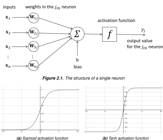
Single neuron cell

A single neuron is composed of layer in artificial neural networks. The structure of a single neuron is shown in Figure 2.1. The inputs are the vectorx= [x1,x2,x3 ... xn],n denotes the number of inputs, the matching weight for the input is the vectorWj= [W1j, W2j,W3j ... Wnj],jis thejthneuron in the layer. The inputs are first multiplied byWj, the temporary result is generated and the bias value is added to the temporary result, b is the bias. Then this result is inputted into the activation function f. The corresponding mathematical form of the forward computation in a single neuron is given in Equation 2.1, whereicounters from 1 ton,yj is the output value of thejthneuron for the inputx.

yj =f ( b+ n ∑ i=1 xiWij ) (2.1) Activation functions

(12)

𝐱𝐱

1

𝐱𝐱

2

𝐱𝐱

3

𝐱𝐱

𝑛𝑛

inputs

weights in the

𝑗𝑗

𝑡𝑡𝑡

neuron

𝐖𝐖

1𝑗𝑗

𝐖𝐖

2𝑗𝑗

𝐖𝐖

3𝑗𝑗

𝐖𝐖

𝑛𝑛𝑗𝑗

𝛴𝛴

𝑦𝑦

𝑗𝑗

activation function

𝑓𝑓

_{output value}

for the

𝑗𝑗

𝑡𝑡𝑡

neuron

b

bias

Figure 2.1.The structure of a single neuron

(a)Sigmoid activation function (b)Tanh activation function

Figure 2.2. Sigmoid and Tanh activation function

Activation functions are a basic component of an artificial neuron. A numerical value is accepted as the input in the activation function. The output is calculated after applying the mathematical calculation. There are a few common activation functions such as sigmoid, Rectified Linear Unit (ReLU)[55] etc.

The Sigmoid function is a common activation function for calculating probability. The mathematical formula of the sigmoid function isSigmoid(x) = 1/(1 +e−x_{). The plotting} of this activation function is shown in Figure 2.2a. It is seen that the sigmoid function takes a real-valued number and maps the input into a range between 0 and 1. In particular, when a large negative value is inputted into the sigmoid function, the output value is near 0. If a large positive value is inputted into the sigmoid function, one value near 1 is generated.

The Tanh function is another non-linearity activation function. The formula of this function is(x) = 2/(

1 +e−2x)

−1. The plotting of this activation function is shown in Figure 2.2b. The output range of the Tanh function is (−1,1). The Tanh activation function is similar with the sigmoid function, which it saturates. However, the output of the Tanh function is zero-centered.

(13)

(a)ReLU activation function (b)Leaky ReLU activation function

Figure 2.3. ReLU and leaky ReLU activation function

The ReLU [36] is a piece-wise linear activation function. The formula of the ReLU acti-vation function isReLU(x) = max(0, x) and it is plotted in Figure 2.3a. It shows that the output value range of the ReLU is in the positive area or zero for any numerical input. The ReLU activation function has two advantages. The first one is that the ReLU function is simple to compute, this feature delivers the benefit on computing speed. The second advantage is that ReLU does not saturate like the Sigmoid or Tanh activation function since the gradient of ReLU is constant. These two advantages lead to fast converging speed when a DNN model with ReLU activation function is trained. One variant of the ReLU function is the leaky ReLU activation function [33]. The mathematical formula of leaky ReLU is given in Equation 2.2. It is plotted in Figure 2.3b. The first improvement of leaky ReLU is that it does not have zero-slope parts. The second improvement is that leaky ReLU has faster training speed than ReLU. Thus, the leaky ReLU is considered as an alternative for the ReLU function.

f(x) = ⎧ ⎨ ⎩ 0.01x forx <0 x forx≥0 (2.2) Neural network

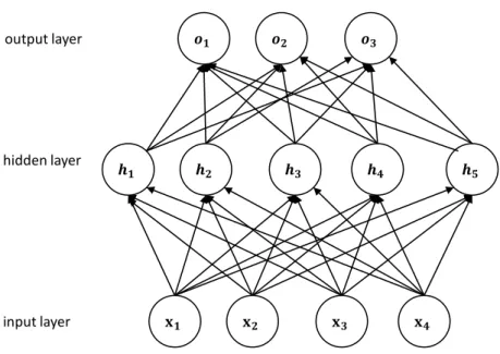
The typical architecture of a neural network consists of input layer, hidden layer and output layer. A classic demonstration of a neural network is the multi-layer perceptron. The architecture of multi-layer perception is shown in Figure 2.4. It shows this multi-layer perception model consists of a input layer, a hidden layer and a output layer. Regarding the architecture of deep neural networks [28], it consists of more that one hidden layers.

2.1.2 Convolutional neural network

Convolutional Neural Network (CNN) is an important category of neural networks. CNN models usually consist of convolutional layers, hidden layers, pooling layers and fully connected layers.

(14)

𝐱𝐱𝟏𝟏 𝐱𝐱𝟐𝟐 𝐱𝐱𝟑𝟑 𝐱𝐱𝟒𝟒 𝒉𝒉𝟏𝟏 𝒉𝒉𝟐𝟐 𝒉𝒉𝟑𝟑 𝒉𝒉𝟒𝟒 𝒉𝒉𝟓𝟓 𝒐𝒐𝟏𝟏 𝒐𝒐𝟐𝟐 𝒐𝒐𝟑𝟑 output layer hidden layer input layer

Figure 2.4.Typical architecture of the multi-layer perceptron

x1 x2 x3 x4

x5 x6 x7 x8

x9 x10 x11 x12

a

b

c

d

ax1 + bx2 + cx5+dx6 ax2+bx3+cx6+dx7 ax3 + bx4 + cx7 + dx8

ax5+bx6+cx9+dx10 ax6+bx7+cx10+dx11 ax7+bx8+cx11+dx12

input in the feature map _kernel

Figure 2.5. Convolution operation illustration

Convolutional layer

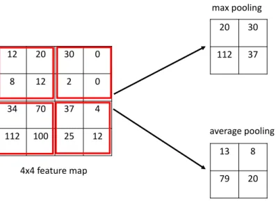
Convolutional layer is the key element for building a CNN model. Through the convolu-tion operaconvolu-tion, features in the convoluconvolu-tional window are learned. In addiconvolu-tion, parameter sharing scheme is applied to reduce the number of parameters when operating the con-volution. A demonstration of the convolution operation in CNN model is shown in Figure 2.5. It shows that the volume size of the feature map is 3×4, the convolution kernel size is 2×2 and the stride step is 1. The dot product is applied to each element. The output volume is generated after the convolution operation. The volume size of the output is 2×3.

(15)

12 20 30 0 8 12 2 0 34 70 37 4 112 100 25 12 20 30 112 37 13 8 79 20 average pooling max pooling 4x4 feature map

Figure 2.6. Max pooling and average pooling operation comparison

Pooling layer

Pooling layer is another important component in CNN models. The pooling operation in CNN is to aggregate the spatial feature. The max pooling and the average pooling operation are the two main pooling operations. The max pooling operation extracts the most obvious feature from the feature map. For example, the max pooling operation can detect edges for the image data. The average pooling operation extracts features in a smooth manner. It takes all values inside the convolutional window and computes the average value out of the window, which indicates that the average pooling operation takes into all values into account. The Figure 2.6 shows the difference between the average pooling and the max pooling operation. In the figure, the size of the feature map is 4 × 4. The convolutional window size is 2 × 2. During the max pooling operation, the largest value in each convolutional window is selected while the average value in each convolutional window is calculated in the average pooling operation.

Common CNN models

During the development of convolutional neural networks, many significant variant CNN models were proposed. AlexNet [26] won the champion in the ImageNet Large Scale Vi-sual Recognition Competition (ILSVRC) [43] 2012 competition. The ImageNet dataset [7] contains 1000 classes images, including dogs, cats, flowers, and planes etc. The task for this competition is to classify images into correct classes. AlexNet model achieved 83.6% the highest accuracy. It decreased 9.4% error rate from the champion model in the pre-vious year. Regarding the architecture of AlexNet, it is a typical modern CNN model, which consists of five convolutional layers, max-pooling layers, three fully connected lay-ers. The VGG-16 model [6] won the ILSVRC champion in 2013. A key contribution of the VGG-16 model was the model depth. The VGG-16 model increased the depth of 8 layers in AlexNet to 16 layers. It was the deepest CNN model in 2013 and the VGG-16 model decreased the error rate to 7.3% in the ImageNet dataset and showed the

(16)

pow-erful learning ability of deep neural networks. Another contribution was the concept of repeating module to construct deep neural networks. This idea of using repeating block was inherited by many other models afterwards. Regarding the model architecture, the VGG-16 model comprised of 13 convolutional layers and 3 fully connected layers. And the size of reception filters for convolution operation was 3×3. Kaiming et al. proposed the ResNet model [12] in 2015. The ResNet model with 50 convolutional layers won the ILSVRC competition in the year. A innovation of ResNet model was that the short-cut operation was introduced to mitigate the gradient vanishing problem in deep neural networks. Deep neural networks become harder to train and suffer gradient vanishing problem when the depth of the model increases. Through the shortcut operation, the gradient in DNN models can be passed to the next layers easier. The shortcut operation becomes the a useful technique for building CNN model later.

2.1.3 Recurrent neural network

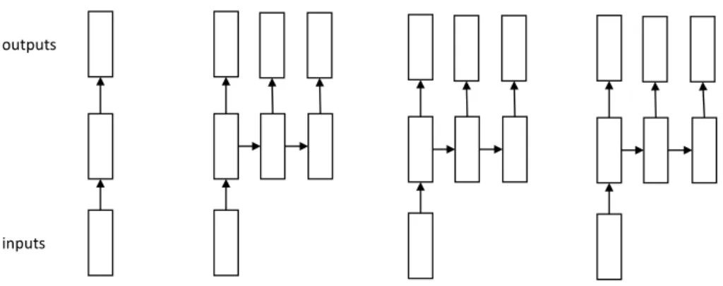
Recurrent Neural Network (RNN) [34] is another important type of deep neural networks. RNN model is good at processing sequence data and text data is an important type of sequence data. RNN model can be categorized into four different types. There are one-to-one RNN model, one-to-many RNN model, to-one RNN model, and many-to-many RNN model. The detailed structure for these four models is illustrated in Figure 2.7. These four models are designed to deal with corresponding specific tasks. The tag prediction task [10] for one sentence in NLP area is the typical scenario for the many-to-many RNN model. Another typical application for the many-to-many-to-many-to-many RNN model is the machine translation task. The sentiment classification task is a representative task for the many-to-one RNN model. In the sentiment classification task, each word in the sentence is considered as one input, the predicted result of the sentiment class for the sentence is the only output.

When comparing to CNN models, a difference between RNN and CNN is the depth of layers. The depth of layers in the CNN model can be deep, in some case, the depth of CNN is over 100. However, the most common depth of layer in RNN model is shallow. The main reason for shallow layers in RNN is that RNN model is unfolding and calculated along with the time steps while CNN model calculate in the space instead.

RNN uses hidden states to store information which is generated in the previous time steps. The typical structure of RNN model unfolding computational graphs along with the time steps is shown in Figure 2.8. In this figure, the vectorxis the input, the vector o is the predicted result, the loss function is L, the true class is y, the h denotes the hidden state, the weight matrix between the input and the hidden state is presented by U. The weight matrix for the connection between the hidden state and the output isV. W denotes the weight matrix between the hidden state in previous time step and the hidden state at current time step. The vectorsx(t−1),x(t),x(t+1) are three inputs at the t−1, t, t+ 1 three different time steps respectively. x(t−1) connects the hidden state

(17)

one to one RNN model one to many RNN model many to one RNN model many to many RNN model inputs

outputs

Figure 2.7. Four types of RNN models

h(t−1) in thet−1time step,o(t−1) _{denotes the output in the}_t₋₁_{time step. The vector} x(t) is the input in thettime step, band c are bias vectors, ϕis the activation function. The mathematical form of calculating the predicted valueois given in Equation 2.3. The total loss for the given sequencexwithyas the targeted values is the sum of the losses over all the time steps.

a(t)=W h(t−1)+U x(t)+b (2.3) h(t)=ϕ ( a(t) ) o(t)=c+V h(t) Long short term memory neural network

LSTM [13] is a well-known type of recurrent neural network and was proposed in 1997. One drawback of traditional RNN is that it is hard to capture the semantic and syntactic relation between two words with long distance in the text sequence data . This problem is known as the short memory issue. Long Short Term Memory neural network (LSTM) can mitigate this problem by using gate control mechanism to learn long term dependency in sentences. Besides, LSTM model can mitigate the gradient exploding problem. During the training phase of RNN model, gradients are usually exploded when the propagation of the gradients feeds forward. The design of the LSTM model overcomes the technical challenges of RNN to deliver on the promise of sequence prediction with neural networks. Regarding the structure of LSTM cell, it is shown in Figure 2.9. Three gates are designed to control the information flow in neural networks, they are the input gate, the output gate and the forget gate respectively. The matrixXt∈Rn×dis the input of the LSTM cell in the ttime step, nis the number of samples, dis the number of dimensions. It is the value

(18)

Figure 2.8.The unfolding recurrent neural network along with time steps [9]

matrix of the input gate in the t time step, Ht−1 is the parameter matrix of the hidden

states in thet−1 time step, the matrixWhi represents the weight matrix between the hidden state and the input gate,bi is the vector of bias parameter in the input gate.Ftis the value matrix of the forget gate in thet time step,Wxf is the weight matrix between the input gate and the forget gate,Whf is the weight matrix between the hidden state and the forget gate,bf is the vector of bias parameter in the forget gate.Otis the value matrix of output gate in thettime step,Wxois the weight matrix between the input gate and the output gate,Who represents the weight matrix between the hidden state and the output gate,bois the vector of bias parameter in the forget gate,ϕis the activation function. The three gate and the hidden states variables use Equation 2.4 to update their values.

It=ϕ(XtWxi+Ht−1Whi+bi) (2.4)

Ft=ϕ(XtWxf +Ht−1Whf +bf)

Ot=ϕ(XtWxo+Ht−1Who+bo) Bidirectional recurrent neural network

In feed-forward recurrent neural network, it is assumed that the syntactic and semantic information of the current word is determined by the previous appearing words. This indicates that the value of variables in the current time step is determined by the variables in the earlier time steps when the computational graph of recurrent neural networks is

(19)

Figure 2.9.LSTM cell structure [56]

unfolding along with the time steps. However, the syntactic and semantic information of a word is determined by both the earlier appearing words and the later appearing words in many situations. Context information is an important factor for deep neural networks in the text classification task, especially in the long text case. For the semantic information, the one-way recurrent neural network only considers the information from the previous appearing texts, not using the information from the latter text. This results in the problem of losing semantic information.

The bidirectional recurrent neural network [44] was proposed to tackle this type of prob-lem. Figure 2.10 illustrates the structure of a bidirectional recurrent neural network. In this figure, the hidden state for the forward direction in thettime step is−H→t∈Rn×h, the hidden state for the backward direction in thettime step is←Ht− ∈_Rn×h_,_n_{is the number} of samples which are inputted to the model, h is the number of hidden neurons, Xt is the matrix of the input value in the t time step, (f) indicates the forward direction, (b) indicates the backward direction in the bidirectional recurrent neural network, ϕ is the activation function,W(_hhf)is the weight matrix between the hidden neurons in the forward direction, W(_xhf) is the weight matrix between the input and the hidden neurons in the forward direction, −Ht→−1 is the parameter matrix of the hidden neurons in the t−1 time

step in the forward direction,b(_hf) is bias parameters in the hidden states in the forward direction. Regarding the backward direction,W(_xhb)is the weight matrix between the input and the hidden neurons in the backward direction, ←Ht−+1 is the parameter matrix of the

hidden neurons in thet+ 1time step in the backward direction,W(_hhb)is the weight matrix between the hidden neurons in the backward direction,b(_hb)is the bias parameters in the hidden neurons in the backward direction. The forward and backward hidden states are computed using Equation 2.5.

−→

(20)

𝐗𝐗𝟏𝟏 𝐗𝐗𝟐𝟐 𝐗𝐗𝐭𝐭−𝟏𝟏 𝐗𝐗𝐭𝐭 … 𝐇𝐇𝟏𝟏 𝐇𝐇𝟐𝟐 𝐇𝐇𝐭𝐭−𝟏𝟏 𝐇𝐇𝐭𝐭 … 𝐇𝐇𝟏𝟏 𝐇𝐇𝟐𝟐 𝐇𝐇𝐭𝐭−𝟏𝟏 𝐇𝐇𝐭𝐭 … 𝐎𝐎𝟏𝟏 𝐎𝐎𝟐𝟐 𝐎𝐎𝐭𝐭−𝟏𝟏 𝐎𝐎𝐭𝐭 …

Figure 2.10.The structure of the bidirectional recurrent neural network

←−

Ht=ϕ(XtW(_xhb)+←H−t+1W(_hhb)+b(_hb))

The forward and backward hidden states,−H→t, ←−

Ht, are concatenated to obtain the hidden stateHt∈Rn×2hin thettime step. The hidden stateHt∈Rn×2his inputted to the output layer, Whq is the parameter matrix in the output layer,bqis the vector of bias parameter in the output layer. The output layer computes the outputOt∈Rn×q with using Equation 2.6,qis the number of outputs.

Ot=HtWhq+bq (2.6)

2.1.4 Optimization algorithms

Objective function

The aim of training a DNN model is to reduce the value of loss function. The optimization algorithms are used to update the value of model parameters to decrease the value of the model objective function. When the training phase ends, the parameters of the model at the time are the parameters that the model learned from the training phase. Objective function is also named loss function in deep neural networks. The value of the objective function is the average value of the calculated losses when the data from the training data set is loaded to train a DNN model. The common form of objective function of a neural network is defined in Equation 2.7,f(xi) is the loss function for thexi sample in the training data set, nis the number of training samples, f(x) is the objective function

(21)

Figure 2.11. Stochastic gradient descent optimization algorithm for the functionf(x) = x2₁+ 2x2₂ [56]

for all n samples. When the feed-forward process for training deep neural networks is completed, the average value of the losses is calculated. Then the back-propagation algorithm is applied to calculate the gradient value of x in layers of DNN models with using Equation 2.8, where∇f(x)is the gradient ofxwith functionf.

f(x) = 1 n n ∑ i=1 f(xi) (2.7) ∇f(x) = 1 n n ∑ i=1 ∇fi(x) (2.8)

Stochastic gradient descent

During training processing, the optimization algorithms are critical for training deep neural networks since the training phase usually takes a few days or longer time to complete. Therefore, the optimization algorithm has an obvious effect on the cost time for the train-ing. There are many optimization algorithms such as Stochastic Gradient Descent (SGD) [4], Adam [22]. In this thesis, SGD is used as the optimization algorithm.

A demonstration of applying SGD is shown in Figure 2.11. The input is a two-dimensional vector,x= [x1,x2], the objective function isf(x) =x21+2x22. SGD optimization algorithm

is used to find the minimal value for this function. The initial position forxis(−5,−2), the iteration for updating xis 20 times. After the 20 times iteration, the functionf(x) finds the minimum point(0,0).

(22)

Figure 2.12. Overfitting in deep neural networks [9]

2.1.5 Back-propagation

Back-propagation [42] is used to compute the gradient in different layers in deep neural networks from the cost function. The information from the loss function is flowed back-wards through back-propagation. Back-propagation exploits the derivative chain rule to compute derivatives. The data is inputted to feed forward propagation to update the value through different layers in DNN model and the value of the loss function is calcu-lated later. When back-propagation is applied in recurrent neural network, the normal form of the back-propagation can not be applied directly since RNN is time sequence model. Therefore, back-propagation through time (BPTT) [54] was introduced for solving this problem. BPTT algorithm is the variant of back-propagation to compute the gradient. The recurrent neural network is required to expand along with the time steps in BPTT to obtain the dependencies in different time steps.

2.1.6 Regularization technique

Overfitting problem

Deep neural networks have strong representation learning ability. In the other hand, the lack of control over the learning process in deep neural networks can lead to the overfitting problem. The overfitting indicates that models have low generalization ability, which results in the bad prediction ability for test data even though the model achieves high performance in training data or validation data. Overfitting occurs when the gap between the training error and testing error is large. The illustration of the overfitting problem is shown in Figure 2.12. This situation indicates that the deep neural network model is trained to have a good fitting ability on the train data instead of learning the data patterns.

(23)

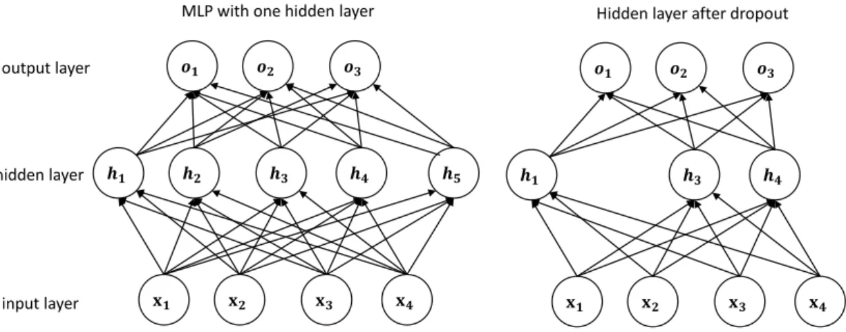
𝐱𝐱𝟏𝟏 𝐱𝐱𝟐𝟐 𝐱𝐱𝟑𝟑 𝐱𝐱𝟒𝟒 𝒉𝒉𝟏𝟏 𝒉𝒉𝟐𝟐 𝒉𝒉𝟑𝟑 𝒉𝒉𝟒𝟒 𝒉𝒉𝟓𝟓 𝒐𝒐𝟏𝟏 𝒐𝒐𝟐𝟐 𝒐𝒐𝟑𝟑 output layer hidden layer input layer 𝐱𝐱𝟏𝟏 𝐱𝐱𝟐𝟐 𝐱𝐱𝟑𝟑 𝐱𝐱𝟒𝟒 𝒉𝒉𝟏𝟏 𝒉𝒉𝟑𝟑 𝒉𝒉𝟒𝟒 𝒐𝒐𝟏𝟏 𝒐𝒐𝟐𝟐 𝒐𝒐𝟑𝟑

MLP with one hidden layer Hidden layer after dropout

Figure 2.13.The structure comparison of MLP with and without dropout technique

neural networks. The common regularization methods include dropout, batch normaliza-tion, parameter norm penalties, early stopping mechanism, multitask learning technique etc.

Dropout

Dropout is a regularization technique to deal with the overfitting problem for DNN mod-els. Dropout [46] technique is considered as a way of approximately combining many different neural networks together in an efficient way. Dropout is explained to drop out neurons in a hidden layer in a neural network. Dropping neural neurons out indicates temporarily removing the neurons and their corresponding incoming and outgoing con-nections in the neural network. The concept of dropout is illustrated in Figure 2.13. When the dropout technique is applied to the hidden layers in the multi-layer perceptron, there is a probability for neurons in the hidden layer to be skipped.

In [46], the authors experimented that convolutional neural network with dropout tech-nique in fully connected layers had 14.32 % error rate in the CIFAR-10 dataset [25] while the original convolutional neural network without applying dropout contained 14.98 % error rate in the CIFAR-10 dataset. The experiments also showed that the model with applying dropout technique reduced the error rate from 43.48 % to 37.20 % in the CIFAR-100 dataset. The authors tested the dropout technique in the ImageNet dataset as well. The best method based on standard vision features achieved 26 % top-5 error rate in the ImageNet dataset at the time. However, the convolutional neural network with applying dropout achieved 16% top -5 test error. These experiments indicated that the dropout technique can improve the generalization ability for deep neural networks.

Batch normalization

Batch normalization [16] is another wide applied technique to improve the generalization ability of DNN. Batch normalization operation is usually inserted after fully connected lay-ers or convolutional laylay-ers and before the activation functions. Through the batch normal-ization operation, the weight values of different layers in neural networks are normalized

(24)

with following 4 steps. The mini-batch inputs areC=[x1, ...xn],nis the number of inputs which are applied to activation functions. The first step of applying batch normalization is to calculate the mean value on the mini-batch inputs with using Equation 2.9, where µC is the mean value onC. Secondly, the variance of the mini-batch inputs is computed

using Equation 2.10, where σ2

C is the variance value onC. The third step is to apply the

normalization with using Equation 2.11, ϵis a constant for numerical stability, the _ˆxi is the normalized value for thexi. The fourth step is using the Equation 2.12 to scale and shift the variable _ˆxi, whereyi is the final batch normalized value of xi. γ and β are two learnable hyper-parameters. µC← 1 n n ∑ i=1 xi (2.9) σ2C← 1 n n ∑ i=1 (xi−µC)2 (2.10) ˆ xi ← xi−µC √ σ_C2+ϵ (2.11) yi←γxˆi+β ≡BatchNormalizationγ,β(xi) (2.12)

In [16], the authors experimented that the effect of batch normalization in the Inception deep neural network [48]. Their experiments showed that the Inception variant with batch normalization achieved 72.7% accuracy while the basic Inception model had 72.2% accu-racy in the ImageNet dataset, which demonstrated that the performance of the Inception V3 model [49] was improved by 0.5% accuracy through the batch normalization tech-nique in the ImageNet dataset. Furthermore, the training time for the Inception model was reduced when the batch normalization technique was applied according to their experi-ments result. A explanation for consuming less training time was that batch normalization can boost the speed of converging for training deep neural networks.

2.2 Natural language processing

2.2.1 Sentiment classification introduction

The objective of sentiment classification is to classify text into different categories ac-curately according to the sentimental polarity expressed from the text. Normally, the sentiment of text is labeled into 3 classes or 5 classes. For the type of 3 classes, the sentiment of a review is classified as negative, neutral or positive. For the 5 classes type, the sentiment for a text is labeled as one of the following class: very negative, negative,

(25)

Table 2.1. Examples of text review for sentiment classification

examples sentiment

“The strange thing is that it works” positive “Shattered image is not complex, it’s just boring and stupid” negative “Far from bewitching, the patience can be tested by the crucible” neutral

neutral, positive or very positive. Table 2.1 shows examples of sentiment classification on reviews.

Use cases for sentiment classification

Sentiment classification has been widely applied in many areas with several applications, such as search engine, text information retrieval, machine reading and understanding etc. Three use cases for applying text classification methods are briefly described. One example is the news category classification task, which text news related to different topics needs to be classified to their correct corresponding topics. There are many differ-ent topics including sports, finance, technology, health etc. Each topic is considered as one class. Sports news should be predicted as the sport category instead of finances. With the help of the text classification technique, users can avoid wasting time on reading unrelated articles. The second example is that sentiment analysis can be used to pre-dict market trends through analyzing customers’ reviews about some specific products. A real example of this application is about Samsung Note 7 battery crisis in 2017. The number of negative sentimental tweets of Samsung in Twitter increased dramatically af-ter the Samsung note 7 bataf-tery crisis happened. Through observing the change of the number of positive and negative sentimental tweets, Samsung company can evaluate the effect of this crisis ahead. Another common usage of sentiment analysis is collecting and analyzing software application reviews [30] [29]. After each update of an applica-tion in iOS or Android operating system, software developers want to know what users think of the newly developed version. Through utilizing the sentiment analysis technique on these application reviews, developers can conclude clear feedback from users’ com-ments. In [32], authors introduced probability-based sentiment classification technique to classify reviews which were collected from mobile phone applications in Apple app store and Google play store. These reviews were classified to four different categories: feature requests, text rating, user experiences and bug reports. Sentiment classification can be applied in the politics area as well. When a new policy is proposed, the government can gather people’s opinion and discussion content from multiple sources to obtain feedback on the new policy. then the government can improve or adjust the policy in the next step.

2.2.2 Word embedding

Word embedding is a type of algorithms which map words or phrases from vocabulary to vectors in numeric values form. Each word is represented by a vector with using word

(26)

Text Language model Statistical methods NNLM word2vec GloVe FastText SVD TF-IDF Bag of words ELMo

Figure 2.14. Overview of word embedding technique

embedding technique. The similarity of different words can be measured by the distance metrics such as calculating cosine similarity. The overview of word embedding technique is shown in the Figure 2.14, the bag of words method is a traditional word embedding technique. The Term Frequency-Inverse Document Frequency (TF-IDF) algorithm and Singular Value Decomposition (SVD) are another two typical statistical methods for gen-erating word vectors. The language model based word embedding methods consider the semantic context information and have many advantages When compared to statistical word embedding technique. For example, the curse of high dimensionality and vector sparsity problem can be mitigated by utilizing the distributed word embedding technique. There are various algorithms to generate word embedding vectors for words in corpus. One knowing work is the Neural Network Language Model (NNLM) [2]. Matthew et al. [39] proposed the Embeddings from Language Models (ELMo) to represent word embed-ding in 2018. In this thesis, three different algorithms are elaborated. The first one is the Word2vec, the second one is the FastText and the third word algorithm is the GloVe. Word2vec

The Word2vec [35] algorithm was first introduced in 2013. The Continuous Bag of Words (CBOW) and the Skipgram are the two variant models for computing word vectors. The Skipgram model predicts a target word with utilizing the nearby appearing words. In contrast, the CBOW model predicts the target word according to the surrounding context. The context is represented with using bag of words method which are contained in a specified size window around the target word. An example for illustrating the difference between the Skipgram and the CBOW model is shown in Figure 2.15. The sentence "I am selling these fine leather jackets" is given and the target word is "fine". The CBOW model predicts the target word with using the information of all the surrounding words, including "selling", "these", "leather", and "jackets". The sum of these word vectors is applied to

(27)

Figure 2.15.The continuous-bag-of-words versus the skipgram method [14]

predict the target word in the CBOW model. The Skipgram model takes a random near word instead of all words to predict the target word. In addition, the Skipgram model had better performance than the CBOW model in general according to the result of the experiments.

A demonstration of the effectiveness of wording embedding is illustrated in Figure 2.16. Two categories of English words are listed in this figure. The first words category is the countries, including "France", "Germany", "Spain" etc. The second category is the corre-sponding capital cities, including "Paris", "Berlin", "Madrid" etc. The word embedding for these English words was trained using the Skipgram model. The 300 dimensional word vectors for these English words were generated after finishing the training process. The Principal Component Analysis (PCA) [18] technique was applied to reduce the dimension size of word vectors from 300 to 2. These two values were treated as the coordinates for words to perform visualization in the figure. It is seen that the English words of these two concepts were clustered separately on each side. The relationship of matching words (countries and capital cities) between these two categories was learned, which indicates that the syntactic and semantic relationship of these words was kept in the word embed-ding form.

GloVe

GloVe [38] is a popular deep neural network based word embedding algorithm. It is a unsupervised learning algorithm for learning word vectors. GloVe was proposed after the Word2vec and had a few changes compared to the Skipgram model. The first change is that the GloVe algorithm adopted square loss instead of cross-entropy loss as the objective function to train model for generating the word embedding. Secondly, the GloVe algorithm considers the global statistics information of the English words based on the whole dataset while Word2vec algorithm only considers the information inside the fix size windows.

(28)

Figure 2.16. Two-dimensional principal component analysis projection of the word vec-tors of countries and corresponding capital cities [35]

Figure 2.17. FastText model architecture for generating the vector representation for a

sentence with ngram featuresx1, . . . ,xN [19]

FastText

The FastText [19] is another common neural network model to generate accurate word vectors. A feature of the FastText model is that the training speed is fast. In the author’s experiments, FastText model only needed 4 seconds to complete one epoch to perform sentiment classification on the Yelp Full review dataset. In contrast, other models needed more than 30 minutes to finish one epoch. The architecture of the FastText model is shown in Figure 2.17. It shows that the model architecture of the FastText was simple, which contains one layer for the word embedding, one hidden layer and one layer for output.

GloVe and FastText are two standard word embedding technique. The comparison for these two algorithms is described in Table 2.2. The training corpus for GloVe are Wikipedia and Gigaword, FastText used Wikipedia as the training corpus. In the aspect of tokens size, GloVe has 6 billion tokens and FastText has 16 billion tokens. One hyper-parameter

(29)

Table 2.2.The comparison between GloVe and FastText word embedding model

model dimensions vocabulary corpus tokens

GloVe 300 400k Wikipedia, Gigaword 6 Billion FastText 300 2520k Wikipedia 16 Billion

for word vectors is the dimensional size. A factor of the syntactic and semantic informa-tion of a word is the dimensional size. In [38], the experiment showed that the accuracy on the word analogy task was higher when the dimensional size of a word is larger. Nor-mally, the 50-dimensional, 100-dimensional and 300-dimensional word embedding size are common. In this thesis, the 300 dimensional size for the word embedding was exper-imented for sentiment classification.

2.2.3 Overview of algorithms for sentiment classification

Zhang et al. [57] proposed a survey on the evolution of the sentiment analysis research area, including the introduction of fundamental algorithms from the perspective of linguis-tics, statistics and computer science. The authors mentioned the challenge in sentiment classification and analyzed why it is a difficult task. Many efforts have been devoted to ex-ploring the sentiment classification from different perspectives. For example, the new text review dataset are introduced and the sentiment classification algorithms are proposed. A perspective of categorizing sentiment classification algorithms is considering the length and form of reviews. Sentiment classification algorithms are divided into three small re-search direction from this perspective: the sentence-level sentiment classification algo-rithms, the paragraph-level sentiment classification algorithm, and the document-level sentiment classification algorithm. In the sentence-level sentiment classification, a whole sentence is treated as the input, the target is to predict the sentimental polarity of the sentence. In the paragraph-level sentiment classification, the vector representation of a paragraph is generated through integrating the sentence vectors, then the sentimental class for the paragraph is predicted. In the document-level sentiment classification, its aim is to classify the whole document text as expressing a positive, neutral or negative opinion. A paragraph is first to do the feature extraction to obtain the vector representa-tion. The paragraph vector is generated by integrating all paragraph vectors afterwards. Moreover, the evolution of text classification algorithms is commonly divided into three main approaches from the perspective of algorithms, linguistic rule-based approach, sta-tistical machine learning approach, and deep neural network-based approach.

The linguistic rule-based algorithm is the earliest applied method to perform sentiment classification task. The linguistic rule-based method utilizes lexicon dictionary to classify the sentiment of text. In this approach, the sentimental words dictionary is first built. The frequencies of different words are calculated. The different weights for words in the sentence are dispatched. Then the final sentimental score for the text is computed. A

(30)

representative algorithm of this method is the VADER [15].

The general process of applying statistical machine learning based algorithms for sen-timent classification contains two steps. The first step is to extract handcrafted features from the text. The second step is to use statistical machine learning classifiers to pre-dict the sentimental class for the specific text. There are many representative works. The common algorithms include Linear Regression (LR), support vector machine [37], Naive Bayes (NB) [41], hidden markov models [40], conditional random fields [47], latent dirichlet allocation [3] etc.

In [37], the authors applied SVM to classify the sentiment of text reviews instead of us-ing topic based sentiment classification methods. The authors’ experimented the uni-grams and biuni-grams features, and the results showed that the SVM with uniuni-grams algo-rithm achieved the state-of-art performance, 82.9% test accuracy on the internet movie database. In [8], the authors proposed a method which classified a term as positive or negative with utilizing the distribution of the frequency count and proportional presence count. Moreover, Konstantinas et al. [23] introduced a new method, which combined the prediction results of SVM and NB classifiers to improve classification performance for sentiment classification.

Deep neural network based algorithms have achieved the state-of-the-art performance in the sentiment classification nowadays. The DNN-based methods have improved the per-formance of sentiment classification algorithm greatly when compared with the other two type algorithms. Moreover, DNN-based methods also simplify the process of performing the sentiment classification task, which integrate the feature extraction and classification steps into a end-to-end processing.

There are many well-known deep neural networks for the text classification task. For example, Kim et al. [21] proposed the Text-CNN model, which applied convolutional neural network on the text. In 2013, Socher et al. [45] proposed a recursive deep neural model for text classification. The recursive deep neural network obtained the highest accuracy in the many text review datasets at the time and it achieved 80.7% accuracy on the fine-grained movie sentiment classification. In 2015, Zhang [59] proposed the level convolutional network to perform the text classification. The character-level convolutional network was the first model to use character instead of word to classify text. Previously, deep neural networks use word-level text input, the authors’ experiment showed that the recurrent neural network had a strong learning representation ability for both characters and words.

2.3 Assessment criteria

There are many metrics to evaluate algorithms for different tasks in NLP area. For ex-ample, a common assessment criteria for the machine translation task is the perplexity criteria [1], which is the value of probability for generating one sentence. The aim of

(31)

train-ing models in the machine translation task is to reduce the value of perplexity. Another example is the BERTScore [58]. The BERTScore was proposed to compute cosine sim-ilarity score to match words between the candidate and references sentence, it can be used to evaluate algorithms in the image captioning and machine translation tasks. To access the performance of algorithms for text classification, four critical metrics are calculated in this thesis, namely precision, recall, accuracy and F1-score. In addition, the confusion matrix is needed to obtain better understanding of the prediction result produced by three DNN models. The brief description of these metrics is described below.

2.3.1 Accuracy and F1-score

Accuracy

The mathematical function for the accuracy metric is given in Equation 2.13.

accuracy= T P +T N

T P +T N +F P +F N (2.13)

• True Positive (TP), it indicates the classifier predicts 1 where the true class is 1. • False Positive (FP), it indicates the classifier predicts 1 where the true class is 0. • True Negative (TN), it indicates the classifier predicts 0 where the true class is 0. • False Negative (FN), it indicates the classifier predicts 0 where the true class is 1. F1-score

A common evaluation method to compare multi-class classification algorithms is to use precision and recall metrics. The mathematical form of precision is given in Equation 2.14. The definition of recall is given in Equation 2.15.

precision= T P

T P +F P (2.14)

recall= T P

T P +T N (2.15)

Precision is also named positive predictive value. Recall is also named sensitivity. High precision means that the classifier predicts almost no inputs as positive unless they are positive. A high recall is explained as the classifier misses almost no positive values. The F1-score is the harmonic mean of precision and recall. The equation of the F1-score

(32)

Table 2.3.The confusion matrix

predicted class

positive negative

actual class positive True Positive (TP) False Negative (FN) negative False Positive (FP) True Negative (TN)

is formulated in Equation 2.16. The F1-score is described as a weighted average value of the precision and recall. The best value of the F1-score is 1 and the worst value is 0. In the multi-class classification task, the average of F1-score for each category with weighting depends on the average parameter. In the experiments, each data sample is treated as the same weight when the F1-score is calculated.

F1= 2∗

precision∗recall

precision+recall (2.16)

2.3.2 Confusion matrix

The confusion matrix is used as a method to visualize the classification result. For the binary classification case, true (positive) and false (negative) are the only two possible outcomes. The Table 2.3 shows the confusion matrix for the binary classification. The prediction result of the algorithm will calculate four outcomes (TP, FN, FP, TN) for each class.

(33)

3 EXPERIMENTS

The whole processes of the experiments were elaborated in this chapter. In the first sec-tion, the TripAdvisor dataset is first introduced, including the main process for making this dataset. The statistics overview of the TripAdvisor dataset and the Stanford Sentiment Treebank dataset (SST) is presented as well. In the second section, the architecture of the three deep neural networks is elaborated. The third section is describing the environ-ment of the experienviron-ments.

3.1 Datasets

3.1.1 TripAdvisor dataset

Data collection

The TripAdvisor dataset1, is made for this thesis. The first step for making the TripAdvisor dataset is collecting the hotel reviews data. A Python web crawling framework, Scrapy [24], was used to crawl hotel review data from the TripAdvisor website. There are two crit-ical reasons for choosing the TripAdvisor website as the raw data source. The first reason is that this website is popular and has a large number of user reviews, which indicates that the reviews data is large enough and the hotel reviews are representative. The sec-ond reason is this website does not have a strong anti-crawling mechanism. Therefore, it has a high probability to crawl the hotel review with not encountering obstacles. The second step is to clean the raw dataset including discarding incomplete hotel reviews. For example, some hotel reviews miss the date of writing the review in the raw data format. The third step for making the dataset is to select the "review" column and the "sentiment class" column. 100000 hotel reviews were picked as the whole dataset in the experiment. Then 70% of the whole dataset was considered as the training set, 10% of the dataset was treated as the validation set, and the remaining 20% was the test set.

A original hotel review in the TripAdvisor website is shown in Figure 3.1. It demonstrates that this hotel review was given a 5 score by a user named "000Glenn" in November 2012. The review content of this data record has three separated paragraphs. The title of this review is "Outstanding". The hotel is "Sofitel Legend The Grand Amsterdam". The text

1_{The TripAdvisor dataset can be accessed through this link:} _{https://drive.google.com/open?id=19T} dLOrqjAQ11lpYRx1r2GcYo79fZXloE

(34)

Figure 3.1.A original hotel review on the TripAdvisor website [50]

format of this hotel review was saved into the JavaScript Object Notation (JSON) format. The stored JSON data is listed in Table 3.1. It shows that a JSON record of the raw hotel review includes the title of the review, the quality level of the hotel, the id of the user, the hotel location, the hotel name, the score rating of the review, reviewing date, the Uniform Resource Locator (URL) of this review, the URL of the hotel, and the review content. To make the text classification dataset, only text reviews and their corresponding classes are needed to keep, other information is dropped. Thus, the "review" and the "score" columns were extracted as the input and class in the experiments.

Overview of the TripAdvisor dataset

In order to classify the sentiment of hotel reviews, the label for each hotel review was set with the reviewers’ score rating. In the experiments, the matching relation between the sentimental scoring and the class is described in Table 3.2.

The distribution of the number of reviews for each class in the TripAdvisor dataset is shown in Figure 3.2. The very positive class has the largest number of hotel reviews among all other four classes, which contains more than 40000 data samples. Thepositive class has over 30000 data samples and it is the second largest number of hotel reviews. However, thevery negativeclass contains less than 10000 data items. This indicates that the data distribution of different sentimental classes hotel review is unbalanced. In this thesis, the problem of unbalanced training data is not considered. The average number of sentences in a hotel review for each class in the TripAdvisor dataset is shown in Figure 3.3. It shows that the a hotel review in thevery negativeclass has the largest number of the sentences on average, which consists of 8.65 sentences for a review. In contrast, a review in the very positiveclass has the least number of the sentences, which has 6.63 sentences. The NLTK [31] library was used as the library for calculating the number of sentences from the whole text review. The average number of words for each sentimental

(35)

Table 3.1.A sample of the raw hotel review data in the TripAdvisor dataset

JSON data value

title Outstanding

hotelStars 5.0

userId 000Glenn

hotelLocation Oudezijds Voorburgwal 197, 1012 EX Amsterdam, The Netherlands

hotelName Sofitel Legend The Grand Amsterdam

score 5 date 2012.11.10 URL https://www.TripAdvisor.com/ShowUserReview s-g188590-d189389-r145091651-Sofitel_Legend_ The_Grand_Amsterdam-Amsterdam_North_Holland_P rovince.html hotelURL https://www.TripAdvisor.com/Hotel_Review-g 188590-d189389-Reviews-Sofitel_Legend_The_Gr and_Amsterdam-Amsterdam_North_Holland_Provinc e.html

review I rate this hotel as the best I’ve stayed in. It occupies a beautiful, historic building sandwiched between two canals in the heart of old ’Dam. It’s at the bottom of the Red Light district, but don’t let that put you off -this is the heart of the old centre, and the hotel’s lo-cality south of the Damstraat bridge which traverses O.Voorburgwal is actually quite peaceful at night. Our room was large and well - appointed with a canal view. The bed, oh the bed. The most comfortable bed I’ve had the pleasure to sleep in. Hermes toi-letries. Spotlessly clean. Service and food are out-standing and what you expect of a hotel of this cali-bre. Concierge was excellent. In summary, I cannot recommend this hotel highly enough. A hotel which richly deserves it’s 5-star rating.

Table 3.2. The matching relation between the sentimental score and class

score sentiment class

1 star very negative 0 2 star negative 1 3 star neutral 2 4 star positive 3 5 star very positive 4

(36)

Table 3.3. The statistics of all sentimental classes in the TripAdvisor dataset

statistics very negative negative neutral positive very positive

number of reviews 5313 6012 15462 36902 46311 number of sentences 8.88 8.65 7.67 6.88 6.63 number of words 176.85 171.11 147.29 124.77 114.02

class in the TripAdvisor dataset is shown in the Figure 3.4. It is seen that the average number of the words for a review in the very negative class is 176.85 while that in the very positiveclass is 114.02.

Table 3.4. Overview of the TripAdvisor dataset, |V| is the vocabulary size, |C| is the

number of classes

data value

dataset TripAdvisor

|C| 5

|V| 99686

average number of sentences in a review 7.08 average number of words in a review 128.46

training set 70000

validation set 10000

testing set 20000

3.1.2 Stanford sentiment treebank dataset

The SST dataset [45] is a common dataset for text classification. All reviews in the SST dataset are related to the movie content. There are two different classification tasks for the SST dataset. The first type is the five-way fine-grained classification and the second one is the binary classification task. For the first type, the five class labels are: very positive,positive,neutral,negative, andvery negative. For the second type, it only contains positive and negative classes. In the experiments, the five-way fine-grained classification type was selected. The overall statistics of the SST dataset is listed in Table 3.6. It is seen that the training set has 8544 data samples, the validation set has 1101 data records and the testing set contains 2210 data records. Five review samples in the SST dataset are listed in Table 3.7. The first column is the movie review, the second column is the sentimental score and the third column is the corresponding class for the sentimental score.

(37)

very negative negative neutral positive very positive 0 10000 20000 30000 40000 num of reviews

Figure 3.2. The distribution of the number of reviews for each class in the TripAdvisor

dataset

very negative negative neutral positive very positive 0 2 4 6 8 num of sentences

Figure 3.3.Average number of sentences per class in the TripAdvisor dataset

very negative negative neutral positive very positive 0 25 50 75 100 125 150 175 num of words

(38)

Table 3.5. Data sample from the TripAdvisor hotel review dataset

hotel reviews class

"just fantastic the staff are amazing every single one of them. The rooms are spacious and very clean. I cant wait to go back!!If you go here book your room on the 4th floor for the added extras. Oh and my 8 year old got free breakfasts on both days bonus.Thankyou for a great stay."

5

"Have stayed at this hotel numerous times, modern hotel, good amenities and rooms are to a good standard. A special mention must go to the staff in the restaurant and bar area both for breakfast and evenings who are friendly and make you feel very welcome. Hotel is positioned 2 minutes form tube station which will take you to Oxford Circus in central London with no changes. Overall I would recommend this hotel both for business or leisure."

4

"The Hotel seems a good distance out form the city centre but the Central Line takes you into Oxford Street in 20 mins and the Hotel is literally 1 minute from Hanger Lane Tube station. The hotel itself is fine. One disappointment was the breakfast in the Club Lounge. Really seemed like minimum effort and probably the poorest I’ve ever had at a Crowne Plaza.Would stay there again because the location is very convenient"

3

"Just poor. I’ve not posted on TA for many years as I forgot my log in details, however this place is so crap I decided to hunt out my details to warn others. The building and facilities are as you’d expect but the staff are just not inter-ested. The check in experience left me wanting to go and play with traffic. They are incompetent and arrogant to the end. Sadly I stay here from time to time with work and will be posting about every bad experience I have, I’m sure there will be more."

2

"So after a very long day I arrived to check in for 4 nights and was informed that although I had a requested a Double room there was only twins available. Great! First time I have slept in a single bed in 20 years. So I head to the room to find stained bedding, dirty curtains, dirty cups and hey that’s life they will have someone look at it the next day.Next day 1 item resolved. And the cups I cleaned and used had been left dirty and the coffee not even replenished (or the chocolates). Glad I only have another 2 nights to endure."

1

Table 3.6. Overall statistics of the SST dataset

data value

dataset Stanford sentiment treebank dataset number of classes 5

vocabulary size 19500

training set 8544

validation set 1101

Sentiment classification with deep neural networks