DEEP NEURAL CLASSIFICATION AND LOGIT REGRESSION BASED ENERGY EFFICIENT ROUTING IN WIRELESS SENSOR NETWORK

2032

A NEW PERMUTATION METHOD FOR SEQUENCE OF

ORDER 2

1_{ABDULLAH AZIZ LAFTA,} 2_{AMMAR KHALEEL ABDULSADAH,} 3_{SAFAA JASIM MOSA}

1,2,3 _{University of Kufa, Faculty of Education for Girls, Department of Computer Science, Najaf, Iraq}

E-mail: 1_{[email protected],} 2_{[email protected],} 3_{[email protected]}

ABSTRACT

Permutation is reordering for a set of objects with taking into consideration the important of order of their locations. In order to increase security performance, this paper presents a new method of permutation for sequence of order 2^8. In this propose method, any information can be converted to the sequence of approximate values between 0 and 255 as a set of blocks. It is needed to build the so called lookup table so that it contains the frequency and positions of the original sequence values. In the experiments, twenty-six image files have been experimented as evidence to the proposed method. In addition, the correlation and entropy measures are computed to test the quality of permutation. All the tests observed that method have significantly effective in reducing the correlation and thereby decreasing the perceptual information of the sequence. Hence, the security is improved.

Keywords: Permutation, Algorithm, Frequency, Sequence, Byte

1. INTRODUCTION

In statistics, permutation is a method to make changes on the elements of samples of data to measure the significant extent of original data. The data sequence can be divided into blocks for analysis purposes [1]. Nowadays, many works in different fields, such as signal processing [2], digital image encryption [3][4][5], bioinformatics [6], neuroimaging [7] and so on use permutation to understand the contents of data to solve a particular problem, such as the highest correlation in data sequence.

The challenge in the permutation field is getting the highest benefits offered from the set of assumptions. Furthermore, a specific type of data adapts with a specific permutation approach. Permutation approaches that are good for textual data may not be suitable for multimedia data [8]. In most of the natural images, the values of the neighboring pixels are strongly correlated. This means that the value of any given pixel can be reasonably predicted from the values of its neighbors [9]. This information is reduced if decreasing the correlation between the image elements using certain permutation process. As a result, when the correlation is decreased, the values of its neighbor’s elements become difficult to predict [3].

In the digital data domain, the smallest element of data is the binary bit in which the data

element (basic unit of information) is represented using the binary number system of ones (1) and zeros (0). Since the byte is a unit of digital information that consists of eight bits, it is permitting the values from 0 to 255. A combination of bytes is referring to one isolated item of information [10].

Data bytes are formed as a set of a sequence of elements which stored at a specific location, for example in a file to be serialized in a file format. The file can be decomposed into blocks or sequences where assuming that the block size is N elements. Small blocks are preferred by some researchers in computer security [4, 5].

The main idea behind the present work is that any source of data, for example a file, can be viewed as an arrangement of N-blocks. The intangible information that presented in that source is due to the correlations among the N-blocks in a given arrangement. This information can be reduced by decreasing the correlation among the N-blocks using the proposed permutation method. In this study, we try to indexing the contents of a sequence into structure that depends on the frequency of each value and the locations of that value within the sequence. The purpose of this approach is to get a complete different structure to the original while retaining the information between the values if a reverse approach has been applied.

2033 methodology in details. Section three shows the experimental results and discussion while the conclusions are summarized in section four.

2. RESEARCH METHODOLOGY

The research methodology is concern with the input sequence of distinct values to build the lookup table for location of these values which help to compute new quantities. These quantities are combined to form the output sequence

2.1. Input Sequence: Definition and Properties

The input for the proposed is a sequence of elements, denoted by S=(V,L). This sequence supposes it contains strong information, which is the orders of its elements, see Figure 1. The sequence has a finite or limited number of elements, say N+1 elements. Here, the maximum possible value could be for N is 255×256+255. As illustrate in figure (1), the two sets V and L are V is the list of all element values appear in S, and L is the list of the corresponding locations of these values where they appear in S.

V={v0,v1,…,vN } and L={l0,l1…,lN} (1)

Also, the input sequence S can be seen as a sequence of ordered pairs of objects as follows:

S={(v0,l0),(v1,l1),…,(vN,lN )} (2)

Define the set B is, B={x: 0 ≤ x ≤ 255} contains only non-negative integers that less than 256. Then vk ∈ V is must be also vk ∈ B.

Each element, say e, in the sequence S has two objects: value, ve ∈ V, and an index or a location,

le ∈ L, i.e. e = (ve, le). The element values are belong

to the set B, i.e. 0 ≤ ve ≤ 255 for any e such that

0 ≤ e ≤ N. That is, V= {ve: ve∈B ∀ 0 ≤ e ≤ N}.

Whereas, the locations of elements are belonging to the range 0⋯N. i.e. L= {le: 0 ≤ le ≤ N ∀ 0 ≤ e ≤ N}.

The element values are explicit information, where element location values are implicit information.

Figure 1: Input Sequence(S)

2.2. Output Sequence: Definition and Properties

The results of the proposed method are four sequences of elements, denoted by QL, RL, QF, and RF. These can be written as follows:

QL= {q0, q1,⋯,qN}and RL={r0,r1,⋯,rN} (3)

QF={q0,q1,⋯,q255 } and RF={r0,r1,⋯,r255 } (4)

Such that, qi ∈ B ∀ qi ∈ QL and

ri ∈ B ∀ ri∈ RL for 0 ≤ i ≤ N. Also, qx ∈ B ∀ qx ∈ QF

and rx ∈ B ∀ rx∈ RF for 0 ≤ x≤ 255.

Where QL and RL are two sequences related to the set L, such that:

li=qi×256+ri for qi∈QL and ri∈RL ∀ 0 ≤ i ≤ N (5)

The other two sequences, QF, and RF are related to frequencies of values in input sequence S. That is, for any value x ∈ B, there is a counter for how many times that value x is repeated in sequence S. Call this value as the frequency of value x, denoted by fx, such that:

fx=qx×256+rx where qx∈QF and rx∈RF ∀ x∈B (6)

Here, if all income values are N values each between v0 and vm, then it should be:

∑ f N 1 (7)

It is important to say that is: F= {f0, f1,⋯,f255} (8)

The set F also is related to set B, by the following:

F={f_x:x∈B} (9)

2.3. Part I Algorithm: definition and steps

In this part, the locations of the distinct value are fetched in order to build a locations table:

The algorithm is composed based on three forward procedures: Build Lookup Table, Generate Output Sequence, and Data Compression.

The first procedure, which called Build Lookup Table algorithm, builds a lookup table called 𝑇 (Figure 2). It is similar to the adjacency list used in graphic representation.

The frequency and location table is a triple set, denoted by (F, V, L). The notation V={v0, …vm}

is the set of all possible income 𝑚 ordered sequence of values could be found. All these values are equal the notation 𝐹 𝑓 . … 𝑓 , is the set of all frequency of each value belong to 𝑉. The 𝐿

𝐿 . … 𝐿 , is set of sets of locations where the

2034 Figure 2: Lookup table T

The main column of the lookup table 𝑇

contains sequentially list of all possible elements of set 𝐵 as shown in figure (2). Hence, one cell for each

𝑥 ∈ 𝐵. The second column, on the left side of the

table 𝑇, is the values of frequency of the elements, which labeled 𝑓. The third part of the table 𝑇 is on the right hand side of the table 𝑇, where there are 256 lists. For each 𝑥 ∈ 𝐵 there is a list, called 𝐿 . The list 𝐿 contains of all possible values of location where the element 𝑥 found in sequence 𝑆. The total number of locations where the element 𝑥 found is 𝑓. If such a location labeled 𝑙 ., then 𝐿

𝑙 . . 𝑙 . . … . 𝑙 . .This part of table could be seen

as a linked list of location values.

Since searching is repeated multiple times on the same sequence of data, we need to speed up the process by building a table for the locations of these data values. So, without losing the locations, the lookup table is work as an index to where these values are in original sequence.

The Build Lookup Table algorithm, as in

Figure 3, comprises two loops. According to the elements of set 𝐵, the first loop will initialize for each element 𝑥 in 𝐵, a frequency counter, 𝑓, to zero, and a location list, 𝐿 , to null, i.e. to be empty. Since there are 256 possible elements in 𝐵, accordingly there are 256 frequency counters, and 256 list pointers. Next, the second loop will get each element

𝑒 in sequence 𝑆. And, according to the element value, 𝑣 , the frequency value, 𝑓, where 𝑥 𝑣 is incremented by one. Also, the element location, 𝑙 , added to the locations list, 𝐿 , where 𝑥 𝑣 .

𝐴𝑙𝑔𝑜𝑟𝑖𝑡ℎ𝑚 𝐵𝑢𝑖𝑙𝑑_𝐿𝑜𝑜𝑘𝑢𝑝_𝑇𝑎𝑏𝑙𝑒 𝑆 𝐹𝑜𝑟 𝑒𝑎𝑐ℎ 𝑥 ∈ 𝐵

𝑀𝑎𝑘𝑒 𝑓𝑜𝑟 𝑥 𝑎 𝑐𝑒𝑙𝑙 𝑖𝑛 𝑇 𝐼𝑛𝑖𝑡𝑖𝑎𝑙𝑖𝑧𝑒 𝑓 𝑡𝑜 𝑧𝑒𝑟𝑜 𝐼𝑛𝑖𝑡𝑖𝑎𝑙𝑖𝑧𝑒 𝐿 𝑡𝑜 𝑛𝑢𝑙𝑙 𝐹𝑜𝑟 𝑒𝑎𝑐ℎ 𝑒 ∈ 𝑆

𝐼𝑛𝑐𝑟𝑒𝑚𝑒𝑛𝑡 𝑓 𝑏𝑦 𝑜𝑛𝑒 𝐴𝑝𝑝𝑒𝑛𝑑 𝐿 𝑏𝑦 𝑙

Return T

Figure 3: Build lookup table

Proposition 1: Build Lookup Table algorithm is correct. The running time is Θ 𝑁 .

Proof: For the correctness observe that the first for-loop iteratively makes a table row for each 0 𝑥 255, where two initialized quantities, 𝑓 and 𝐿 , are located. The next for-loop iteratively get each element in sequence S, increments by one a specific frequency quantity that was initialize by the first-loop, and append a specific list, which also was initialize by the first-loop, according to the testing of the value of that element. Each iteration of both loops, the algorithm updates its local data. So they are both able to perform the computation correctly.

For the complexity observe that the first for-loop is executed Θ 256 times, and the second for-loop is executed Θ 𝑁 . Totally, algorithm has a running time is Θ 𝑁 .

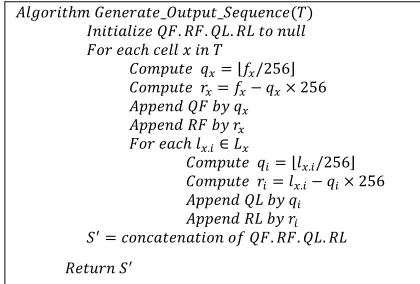
The next work is done by Generate Output Sequence algorithm (figure 4). This algorithm used the lookup table 𝑇 in order to generate the output sequence, called 𝑆. This sequence is a result of a concatenate of the four sequence GF, RF, QL and RL, as shown in the figure (5). So, this algorithm firstly makes these sequences and then finally joins them in one sequence.

𝐴𝑙𝑔𝑜𝑟𝑖𝑡ℎ𝑚 𝐺𝑒𝑛𝑒𝑟𝑎𝑡𝑒_𝑂𝑢𝑡𝑝𝑢𝑡_𝑆𝑒𝑞𝑢𝑒𝑛𝑐𝑒 𝑇 𝐼𝑛𝑖𝑡𝑖𝑎𝑙𝑖𝑧𝑒 𝑄𝐹. 𝑅𝐹. 𝑄𝐿. 𝑅𝐿 𝑡𝑜 𝑛𝑢𝑙𝑙 𝐹𝑜𝑟 𝑒𝑎𝑐ℎ 𝑐𝑒𝑙𝑙 𝑥 𝑖𝑛 𝑇

𝐶𝑜𝑚𝑝𝑢𝑡𝑒 𝑞 ⌊𝑓 /256⌋ 𝐶𝑜𝑚𝑝𝑢𝑡𝑒 𝑟 𝑓 𝑞 256 𝐴𝑝𝑝𝑒𝑛𝑑 𝑄𝐹 𝑏𝑦 𝑞

𝐴𝑝𝑝𝑒𝑛𝑑 𝑅𝐹 𝑏𝑦 𝑟 𝐹𝑜𝑟 𝑒𝑎𝑐ℎ 𝑙. ∈ 𝐿

𝐶𝑜𝑚𝑝𝑢𝑡𝑒 𝑞 ⌊𝑙./256⌋

𝐶𝑜𝑚𝑝𝑢𝑡𝑒 𝑟 𝑙. 𝑞 256

𝐴𝑝𝑝𝑒𝑛𝑑 𝑄𝐿 𝑏𝑦 𝑞 𝐴𝑝𝑝𝑒𝑛𝑑 𝑅𝐿 𝑏𝑦 𝑟 𝑆 𝑐𝑜𝑛𝑐𝑎𝑡𝑒𝑛𝑎𝑡𝑖𝑜𝑛 𝑜𝑓 𝑄𝐹. 𝑅𝐹. 𝑄𝐿. 𝑅𝐿

𝑅𝑒𝑡𝑢𝑟𝑛 𝑆

Figure 4: Generate output sequence

The Generate Output Sequence algorithm start by initializes each set of 𝑄𝐹. 𝑅𝐹. 𝑄𝐿. 𝑎𝑛𝑑 𝑅𝐿

to null, or make an empty set for each. Next, algorithm works top-down on table 𝑇, for each cell

𝑥 in that table, it computes the quantities 𝑞 and 𝑟

from the frequency counter of 𝑥, 𝑓. These computations using the following formulas:

2035 Which yields two quantities in range

0 ⋯ 255. Then, the values 𝑞 and 𝑟 will be added to

the sets 𝑄𝐹 and 𝑅𝐹, respectively. The next step in the procedure is working with the locations list of 𝑥,

𝐿 . Now, each location value 𝑙 . in locations list of 𝑥, 𝐿 , is converted to two quantities 𝑞 and 𝑟, using the following formulas:

𝑞 . _{𝑎𝑛𝑑 𝑟 𝑙}

. 𝑞 256 (11)

Also, we yields two quantities in range

0 ⋯ 255. Then, the values 𝑞 and 𝑟 will be added to

the sets 𝑄𝐿 and 𝑅𝐿, respectively.

Figure 5: Generate output sequence S’

Since, the original sequence 𝑆 has 𝑁 1

elements, our final sequence 𝑆 (figure 5) has more elements. That is because we use two sequences 𝑄𝐹

and 𝑅𝐹, each of length 256, and two sequences 𝑄𝐿

and 𝑅𝐿, each of length 𝑁 1. Which yields a sequence 𝑆 of totally size equal to

2 256 2 𝑁 1 . When calculate the length

of the two sequences, as shown in figure 6, an increasing in length of elements to double and half. Also, the ratio of the sequence 𝑆 length to the sequence 𝑆 length is 1:2.0078. Therefore, we use a data compression approach to enforce a solution for the increasing length problem.

Since, our research not concern to a specific algorithm for data compression. This step is assumed as a practical work, and depends on the data that is used for testing.

|𝑆| 𝑁 1 255 256 255 255 256 1 1

256 1 256 1 1

256 1 1

256 2

|𝑆 | 2 256 2 𝑁 1

2 2 2 2

2 2

|𝑆 𝑆|

2 2 2

2 2 ∙ 2 2

2 2 2 1

= 2 2 Figure 1: Calculation of sequence lengths

Proposition2: Generate Output Sequence algorithm is correct. The running time is Θ 𝑁 .

Proof: For the correctness observe that the outer for-loop iteratively uses all quantities on all 256 table 𝑇 rows. In each iteration, the 𝑞 and 𝑟 values are computed and then update the two pointers 𝑄𝐹

and 𝑅𝐹. The inner for-loop computes 𝑞 and 𝑟 for each quantity inside 𝐿 , and then update the two pointers 𝑄𝐿 and 𝑅𝐿. This work is always done by the iterator 𝑥 which it is belong to 0.255 . The four list

𝑄𝐹, 𝑅𝐹, 𝑄𝐿 and 𝑅𝐿, are all of a fixed length, so the process of concatenate them in one list, 𝑆, is simply and done directly when see them as pointers for specific starting location in sequence 𝑆 .The total work is:

∑ ∑∈ Θ 1 ∑ Θ 𝑓 Θ 𝑁 (12)

2.4. Part II Algorithm: Definition and Steps

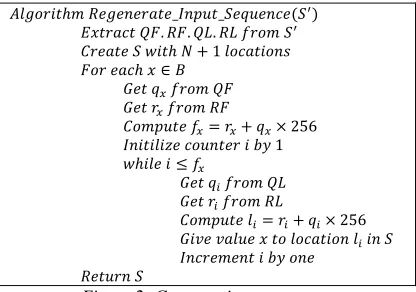
In the opposite direction, after removing the compression, working on reproducing the original sequence S from the generated sequence S is simple. This procedure called Regenerate Input Sequence algorithm, as shown in figure 7. Starting with extracting the four sequences QF. RF. QL and RL

from S. This step is assumed to be strictly reversing for concatenation step in the Generate Output Sequence algorithm.

𝐴𝑙𝑔𝑜𝑟𝑖𝑡ℎ𝑚 𝑅𝑒𝑔𝑒𝑛𝑒𝑟𝑎𝑡𝑒_𝐼𝑛𝑝𝑢𝑡_𝑆𝑒𝑞𝑢𝑒𝑛𝑐𝑒 𝑆 𝐸𝑥𝑡𝑟𝑎𝑐𝑡 𝑄𝐹. 𝑅𝐹. 𝑄𝐿. 𝑅𝐿 𝑓𝑟𝑜𝑚𝑆 𝐶𝑟𝑒𝑎𝑡𝑒 𝑆 𝑤𝑖𝑡ℎ 𝑁 1 𝑙𝑜𝑐𝑎𝑡𝑖𝑜𝑛𝑠 𝐹𝑜𝑟 𝑒𝑎𝑐ℎ 𝑥 ∈ 𝐵

𝐺𝑒𝑡 𝑞 𝑓𝑟𝑜𝑚 𝑄𝐹 𝐺𝑒𝑡 𝑟 𝑓𝑟𝑜𝑚 𝑅𝐹

𝐶𝑜𝑚𝑝𝑢𝑡𝑒 𝑓 𝑟 𝑞 256 𝐼𝑛𝑖𝑡𝑖𝑙𝑖𝑧𝑒 𝑐𝑜𝑢𝑛𝑡𝑒𝑟 𝑖 𝑏𝑦 1 𝑤ℎ𝑖𝑙𝑒 𝑖 𝑓

𝐺𝑒𝑡 𝑞 𝑓𝑟𝑜𝑚 𝑄𝐿 𝐺𝑒𝑡 𝑟 𝑓𝑟𝑜𝑚 𝑅𝐿

𝐶𝑜𝑚𝑝𝑢𝑡𝑒 𝑙 𝑟 𝑞 256 𝐺𝑖𝑣𝑒 𝑣𝑎𝑙𝑢𝑒 𝑥 𝑡𝑜 𝑙𝑜𝑐𝑎𝑡𝑖𝑜𝑛 𝑙 𝑖𝑛 𝑆 𝐼𝑛𝑐𝑟𝑒𝑚𝑒𝑛𝑡 𝑖 𝑏𝑦 𝑜𝑛𝑒

𝑅𝑒𝑡𝑢𝑟𝑛 𝑆

Figure 2: Generate input sequence

Remember that 𝑆 〈𝑉. 𝐿〉. After done the extracting work correctly, an empty sequence 𝑆 is created with 𝑁 1 locations. That is, the set 𝐿 is accomplished. Then we need to accomplish the set

𝑉. Remember that all element values of set 𝑉 are elements of set 𝐵. The sequence 𝑆 are now an information of the distribution of set 𝐵 elements within locations of sequence 𝑆. In order to fill these locations by their values, we use the same approach of take 𝑥 from table 𝑇 in the Generate Output Sequence algorithm. Accordingly, in a sequential manner, for each 𝑥 ∈ 𝐵, we get 𝑞 value from sequence 𝑄𝐹, and get 𝑟 from sequence 𝑅𝐹, in order to compute the frequency counter of 𝑥, 𝑓, using the following formula:

𝑓 𝑟 𝑞 256 (13)

This will allow us to determine how many elements in 𝑆 that must be given the value 𝑥. Now, we need to determine which element locations to filled by 𝑥. So, there are 𝑓 elements taken from the

𝑞   

𝑞 𝑞 𝑟 𝑟    𝑟 𝑞 𝑞    𝑞 𝑟 𝑟    𝑟

2036 two sequence 𝑄𝐿 and 𝑅𝐿 that are of respect to the value 𝑥. Using a loop counter 𝑖 to control how many time to repeat the taken elements process from the sequence 𝑄𝐿 and 𝑅𝐿. With each value 𝑞 taken from

𝑄𝐿, followed by a value 𝑟 taken from 𝑅𝐿, a location value 𝑙 is computed by the following formula:

𝑙 𝑟 𝑞 256 (14)

Hence, the location 𝑙 in sequence 𝑆 is filled by the value of 𝑥. This work will continue until all element locations of S are filled by their values

.

Proposition 3: Regenerate Input Sequence algorithm is correct. The running time is Θ 𝑁 . Proof: For the correctness observe that the four list

𝑄𝐹, 𝑅𝐹, 𝑄𝐿 and 𝑅𝐿, are all of a fixed length, so the process of extracting them from 𝑆, is simply done by determine a starting pointer for each. In the other hand, the length of the retrieved sequence 𝑆 is known be 𝑁 1. The outer for-loop iteratively uses 𝑄𝐹and

𝑅𝐹. In each iteration, 𝑞 and 𝑟 are retrieved from

𝑄𝐹and 𝑅𝐹, respectively, in concurrent way for each

0 𝑥 255, in order to compute 𝑓. Next, the inner while-loop, iteratively reads from 𝑄𝐿 and 𝑅𝐿

concurrently two values, 𝑞 and 𝑟, respectively, to compute the location 𝑙, in which the current value of iterator 𝑥 to be written. Here, the iterator 𝑖, 1 𝑖 𝑓, control when to stop reading from 𝑄𝐿 and

𝑅𝐿.

The total time work is the same as it for Generate Output Sequence algorithm that time complexity computed as follows:

∑ ∑∈ Θ 1 ∑ Θ 𝑓 Θ 𝑁 (15)

Proposition 4: The time complexity for all three algorithms Build Lookup Table, Generate Output

Sequence, and Regenerate Input Sequence is Θ 𝑁 ,

where 𝑁 related to the size of sequence 𝑆.

Proof: The working time, the summation of the three algorithms running time, Θ 𝑁 Θ 𝑁 Θ 𝑁 , is

Θ 𝑁 .

3. RESULTS AND DESCUSSION

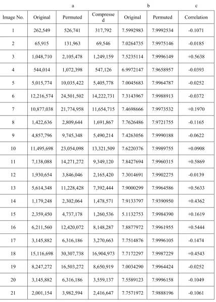
The proposed scheme has been implemented in the C# language and Microsoft Excel 2016 with several test images. Image files are used as a source for correlated data. Some results applied on the TIF format images are below. In the histograms of the permuted elements the nearly uniform distribution of elements values is achieved. In Table 1, 10 of 26 sample tests have been experimented as image files for input sequences. The histograms of permuted sequence are shown in

permutation histogram column. Also, Table 1 presents the column of the compressed permutation sequence histogram. The size in KB for original, permuted, and compressed files listed in Table 2(a). Information entropy is defined as the average amount of information produced by a source of data. Entropy is a measure of uncertainty. High entropy means the data has high variance and thus lot of information is included. The entropy measures of the original blocks and the produced blocks are shown in Table 2 (b). The correlation coefficients between the original sequence and the permutated sequence for each sample are shown in Table 2 (c). The samples are selected according to the differences in the original histogram, as illustrated in appendix I.

4. CONCLUSION

A simple to implement yet effective method has been proposed in this paper for elements permutation taken from files using element frequency and locations permutation method. The main idea is that the strong information in a file can be reduced by decreasing the correlation among the elements using element frequency and locations permutation method. This paper has presented as a method for uniform permutations for image data components. The intelligible information present in an image is due to the correlation among the image elements in a given arrangement. The experimental results have shown that the process of dividing and using frequency-location permutation of image blocks resulted in a lower correlation, a higher entropy value, and a more uniform histogram. Furthermore, the permutation process refers to the operation of dividing and replacing an arrangement of the original image, and thus the generated one can be viewed as an arrangement of blocks.

REFERENCES

[1] Pesarin F, Salmaso L. Permutation tests for complex data: theory, applications and software: John Wiley & Sons. 2010.

[2] Amishima T, Okamura A, Morita S, Kirimoto T. Permutation method for ICA separated source signal blocks in time domain. IEEE Transactions on Aerospace and Electronic Systems. 2010;46(2):899-904.

2037 [4] Mitra A, Rao YS, Prasanna S. A new image

encryption approach using combinational permutation techniques. International Journal of Computer Science. 2006;1(2):127-131.

[5] Sheri PK, Murthy AT. Advanced Image Encryption using Combination of Permutation. International Journal of Emerging Engineering Research and Technology. 2015;3(4):52-59.

[6] Barry WT, Nobel AB, Wright FA. Significance analysis of functional categories in gene expression studies: a structured permutation approach. Bioinformatics. 2005;21(9):1943-1949. [7] Winkler AM, Ridgway GR, Webster MA,

Smith SM, Nichols TE. Permutation inference for the general linear model. Neuroimage. 2014;92:381-397.

[8] Hardiya P, Gupta R. Image Encryption Based on Pixel Permutation and Text Based Pixel Substitution. IJSRD. 2014;2(7):142-145.

[9] Younes MAB, Jantan A. An image encryption approach using a combination of permutation technique followed by encryption. International journal of computer science and network security. 2008;8(4):191-197.

2038

Appendix I

Table 1: The experimented samples

2039

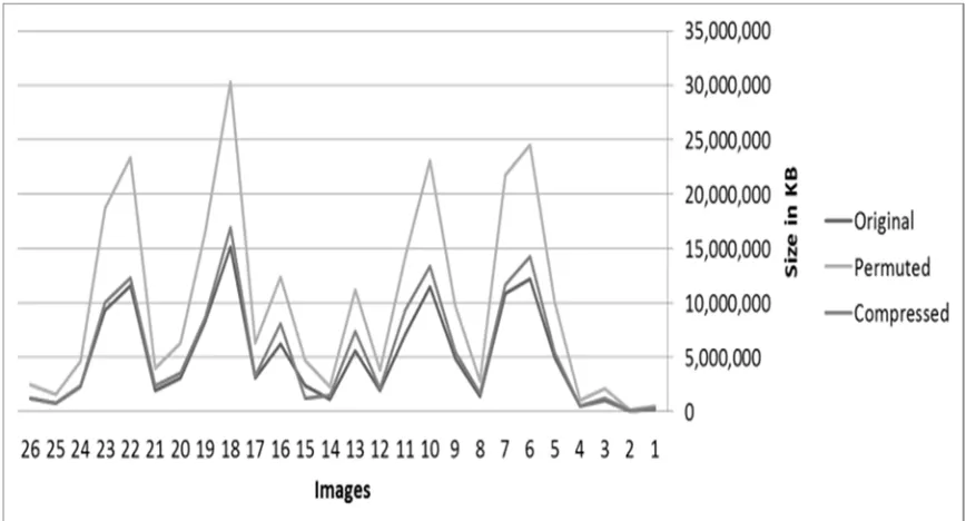
Table 2: (a) Size in KB for orginal, permuated, and compressed files (Figure 8).

(b) Entropy results for orginal elements and the corresponding permuted elements (Figure 9). (c) Correlation between original and permuted sequences (Figure 10).

a b c

Image No. Original Permuted Compresse_d Original Permuted Correlation

1 262,549 526,741 317,792 7.5992983 7.9992534 -0.1071

2 65,915 131,963 69,546 7.0264735 7.9975146 -0.0185

3 1,048,710 2,105,478 1,249,159 7.5235114 7.9996149 +0.5638

4 544,014 1,072,398 547,126 6.9972147 7.9658957 -0.0393

5 5,015,774 10,035,422 5,405,778 7.0045683 7.9964787 -0.0252

6 12,216,574 24,501,502 14,222,731 7.3143967 7.9988913 -0.0372

7 10,877,038 21,774,958 11,654,715 7.4698666 7.9973532 +0.1970

8 1,422,636 2,809,644 1,691,867 7.7626486 7.9721755 -0.1165

9 4,857,796 9,745,348 5,490,214 7.4263056 7.9990188 -0.0622

10 11,495,698 23,054,098 13,321,509 7.6220376 7.9989755 +0.0908

11 7,138,088 14,271,272 9,349,120 7.8427694 7.9960315 +0.5869

12 1,930,654 3,846,046 2,165,420 7.3014691 7.9902275 -0.0139

13 5,614,348 11,228,428 7,392,444 7.9000299 7.9964586 +0.5633

14 1,179,248 2,302,064 1,478,571 7.9133797 7.9390950 +0.4362

15 2,359,450 4,737,178 1,260,536 5.1132753 7.9984390 +0.1619

16 6,211,560 12,420,072 8,148,287 7.8877972 7.9961955 +0.5444

17 3,145,882 6,316,186 3,270,663 7.7514876 7.9996105 -0.1474

18 15,116,698 30,307,738 16,904,973 7.7172297 7.9987229 +0.4543

19 8,247,272 16,503,272 8,650,919 7.0034290 7.9964424 -0.0252

20 3,145,882 6,316,186 3,559,137 7.5589123 7.9996158 -0.1049

2040

22 11,614,618 23,305,114 12,281,158 7.7910437 7.9992485 +0.0721

23 9,313,096 18,691,912 10,031,677 7.3657841 7.9992167 -0.1040

24 2,339,434 4,651,114 2,419,407 7.2934555 7.9856562 -0.0505

25 786,572 1,579,148 814,081 6.6649040 7.9992782 -0.0424

26 1,259,596 2,514,508 1,206,806 7.1949384 7.9933105 -0.0232