Feature Selection using Genetic Algorithms

(1)

San Jose State University

SJSU ScholarWorks

Master's Projects Master's Theses and Graduate Research

Spring 2018

Feature Selection using Genetic Algorithms

Vandana Kannan

San Jose State University

Follow this and additional works at:https://scholarworks.sjsu.edu/etd_projects Part of theComputer Sciences Commons

This Master's Project is brought to you for free and open access by the Master's Theses and Graduate Research at SJSU ScholarWorks. It has been accepted for inclusion in Master's Projects by an authorized administrator of SJSU ScholarWorks. For more information, please contact [email protected].

Recommended Citation

Kannan, Vandana, "Feature Selection using Genetic Algorithms" (2018).Master's Projects. 618. DOI: https://doi.org/10.31979/etd.6mq4-cp5p

(2)

Feature Selection using Genetic Algorithms

A project Presented to

The Faculty of the Department of Computer Science San José State University

In Partial Fulfilment

Of the Requirements for the Degree Master of Science

by

Vandana Kannan May 2018

(3)

(4)

The Designated Project Committee Approves the Project Titled Feature Selection using Genetic Algorithms

by

Vandana Kannan

APPROVED FOR THE DEPARTMENT OF COMPUTER SCIENCE San José State University

May 2018

Dr. Sami Khuri Department of Computer Science Dr. Katerina Potika Department of Computer Science

(5)

ABSTRACT

Feature Selection using Genetic Algorithms by Vandana Kannan

With the large amount of data of different types that are available today, the number of features that can be extracted from it is huge. The ever-increasing popularity of multimedia applications, has been a major factor for this, especially in the case of image data. Image data is used for several applications such as classification, retrieval, object recognition, and annotation. Often, utilizing the entire feature set for each of these activities can be not only be time consuming but can also negatively impact the performance.

Given the large number of features, it is difficult to find the subset of features that is useful for a given task. Genetic Algorithms (GA) can be used to alleviate this problem, by searching the entire feature set, for those features that are not only essential but improve performance as well. In this project, we explore the various approaches to use GA to select features for different applications, and develop a solution that uses a reduced feature set (selected by GA) to classify images based on their domain/genre.

The increased interest in Machine Learning applications has led to the design and development of multiple classification algorithms. In this project, we explore 3 such classification algorithms – Random Forest (RF), Support Vector Machine (SVM), and Neural Networks (NN), and perform 10-fold cross-validation with all 3 methods. The idea is to evaluate the performance of each classifier with the reduced feature set and analyze the impact of feature selection on the accuracy of the model. It is observed that the RF is insensitive to feature selection, while SVM and NN show considerable improvement in accuracy with the reduced feature set.

(6)

The use of this solution is demonstrated in image retrieval, and a possible application in image tampering detection is introduced.

(7)

ACKNOWLEDGEMENTS

I would like to thank my project advisor Dr. Sami Khuri, for his continuous support and encouragement throughout this project. I would also like to thank my

committee members, Dr. Katerina Potika and Mr. Kevin Smith for their time and support. Special thanks to Dr. Natalia Khuri for her valuable inputs and guidance throughout the

(8)

TABLE OF CONTENTS

CHAPTER 1 ... 1

Introduction ... 1

CHAPTER 2 ... 4

Image feature extraction ... 4

2.1 Color models ... 4 2.2 Image features ... 7 CHAPTER 3 ... 24 Genetic Algorithms ... 24 CHAPTER 4 ... 27 Feature Selection ... 27 CHAPTER 5 ... 31 Classification ... 31 5.1 Supervised learning ... 32 5.2 Cross-validation ... 32 5.3 Classification models ... 34 CHAPTER 6 ... 39

Experiments and Results ... 39

6.1 Applications ... 39

(9)

6.4 Results ... 43

CHAPTER 7 ... 50

Conclusion and Future Work ... 50

REFERENCES ... 52

(10)

LIST OF FIGURES

Figure 1 RGB color model ... 5

Figure 2 HSV model ... 6

Figure 3 Features of an image ... 8

Figure 4 Sample image to demonstrate feature extraction ... 11

Figure 5 3´3´5 histogram in the HSV color space of the sample image in Figure 4 ... 14

Figure 6 GLCM adjacency directions ... 15

Figure 7 An example of LBP ... 16

Figure 8 LBP histogram of the sample image in Figure 4 ... 17

Figure 9 Gabor filter applied on the sample image in Figure 4 ... 18

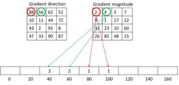
Figure 10 An example of HOG ... 20

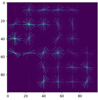
Figure 11 HOG image of the sample image in Figure 4 ... 21

Figure 12 Bilateral filtering applied to the sample image in Figure 4 ... 22

Figure 13 Particle size distribution of the sample image in Figure 4 ... 23

Figure 14: Pattern spectrum of the sample image in Figure 4 ... 23

Figure 15 Simple GA ... 26

Figure 16 Supervised learning ... 32

Figure 17 Cross-validation ... 33

Figure 18 Two classes - Green and Orange ... 34

Figure 19 (a) Linear model (b) Hierarchical model (c) Non-linear model ... 35

Figure 20 (a) Linear SVM (b) Non-linear SVM ... 36

Figure 21 A Random Forest ... 37

(11)

Figure 23 Application of the proposed classifier in theme-based image retrieval ... 40

Figure 24 PACS dataset used for domain generalization ... 42

Figure 25 Art vs Photo: 10-fold ROC curve for RF with Reduced and Full Feature set ... 44

Figure 26 Art vs Photo: 10-fold ROC curve for SVM with Reduced and Full Feature set ... 44

Figure 27 Art vs Photo: 10-fold ROC curve for NN with Reduced and Full Feature set ... 45

Figure 28 Cartoon vs Photo: 10-fold ROC curve for RF with Reduced and Full Feature set ... 46

Figure 29 Cartoon vs Photo: 10-fold ROC curve for SVM with Reduced and Full Feature set .. 46

Figure 30 Cartoon vs Photo: 10-fold ROC curve for NN with Reduced and Full Feature set ... 47

Figure 31 (a) Accuracy comparison: Art vs Photo (b) Accuracy comparison: Cartoon vs Photo ... 47

Figure 32 Test Image 1 [39] ... 59

Figure 38 Test image 7 [41] ... 61

(12)

Figure 45 Test Image 14 [44] ... 65 Figure 46 Test Image 15 [44] ... 65

(13)

LIST OF TABLES

TABLE I Summary of features extracted ... 10

TABLE II Color moments of the sample image in Figure 4 ... 13

TABLE III Haralick features of the sample image in Figure 4 ... 16

TABLE IV (Mean, variance) extracted for each Gabor kernel ... 19

TABLE V Summary of GA Parameters used for Feature Selection ... 30

TABLE VI Comparing accuracies using the T-test ... 49

(14)

(15)

CHAPTER 1 Introduction

A feature is a property or an attribute of data that can be used by algorithms, such as, in the field of machine learning to obtain useful information from datasets. Every datum in an application has some features. For a given application, all features that are extracted or subset of them, are used to obtain an actionable result.

With the increase in data available at our disposal, plus tens to hundreds of features available for different datasets, the complexity of the system increases not only in terms of understanding data, but in terms of resource utilization and system performance. While the size of the dataset cannot be controlled, the feature set can be reduced to include only relevant and unique features so that the overall performance increases and resource utilization decreases [1]. Redundant or irrelevant features may be of the form of correlated features in which there is dependency between them. The dependent features may not provide any extra information or have an impact on the output. This means that eliminating such a feature does not affect the total information content. In some cases, such features may introduce a bias in the system and thus affect the performance. Given that there may be N features possible for a dataset, there may be 2N combinations of features to test to find out which features contribute positively to the outcome of the problem. Evolutionary algorithms such as Genetic Algorithms (GA), can be used for feature selection, where a subset of features must be found from a very large search space.

In the smartphone era, the apps related to capturing or sharing multimedia content have gained popularity. Given the mass multimedia sharing that takes place on the Internet, it is of no surprise that there are large troves of image/video/audio data readily available for use. Particularly, images

(16)

have been used in various applications such as, classification, retrieval, object recognition, and annotation. The fact that images are complex data is proven by the number of features that can be extracted from an image to represent it. The features range from the basic pixel colors to the more complex texture and contour features. It therefore becomes important to make use of feature selection techniques to select only the necessary features for a given application.

Through this work, we investigate the downside of considering huge number of features, by implementing a GA-based feature selection solution, and utilizing the same in an application to classify images based on its genre/domain. Images generally belong to 4 domains: photographs, paintings, cartoons, and sketches [2]. Identifying an image’s genre not only gives the user an idea about the type of the image, but also finds applications in digital forensics, spam analysis, image retrieval, among others.

The aim of this work is to analyze existing work that uses evolutionary algorithms for feature selection, propose a new GA-based solution for feature subset selection, and apply the proposed solution to classify photographs, cartoons, and paintings. The motivation behind selecting these specific classifications is to enable theme-based image retrieval and image tampering detection. The rest of the report is organized as follows:

Chapter 2 explains the various features that have been extracted with the help of a sample image from the dataset considered for this project,

Chapter 3 gives an introduction about GA and the parameters set for the experiments in this project,

Chapter 4 investigates the methods of feature selection and previous work on using GA for feature selection,

(17)

Chapter 5 introduces the concept of classification as a form of supervised learning and explains 3 different classification models that are used in this project,

Chapter 6 highlights possible applications of the proposed solution, references the dataset used for training, and summarizes the results of the experiments,

(18)

CHAPTER 2

Image feature extraction

Feature extraction is the process of parsing input data, in the form of text, image or audio, to find out characteristics that can uniquely represent the data. For example, for audio data, possible features could be sampling rate, pitch, amplitude, duration, etc. Similarly, for image data considered in this work, some examples of features would be mean color, aspect ratio, etc.

2.1 Color models

Color models are mathematical models used to represent colors of an image. This representation is generally a tuple of 3 to 4 values and is independent of devices. Some examples of color models are RGB, CMY, etc. Color spaces on the other hand, represent the colors that can be visualized, for example, aRGB.

Color models can be classified into 3 types [3]:

i) Hardware-based models: Depend on the specifications of the TV monitor, color printer, etc. Example: RGB, CMY, and YIQ.

ii) User-based models: Based on human perception. Represents Hue, Saturation, and Brightness. Example: HSB, HSV, etc.

iii) Hardware-independent models: Color signals are independent of devices. Typically used for transmission over networks. Example: CIE.

For the solution proposed in this work, only Red, Green, Blue (RGB) and Hue, Saturation, Value (HSV) color models are explored.

(19)

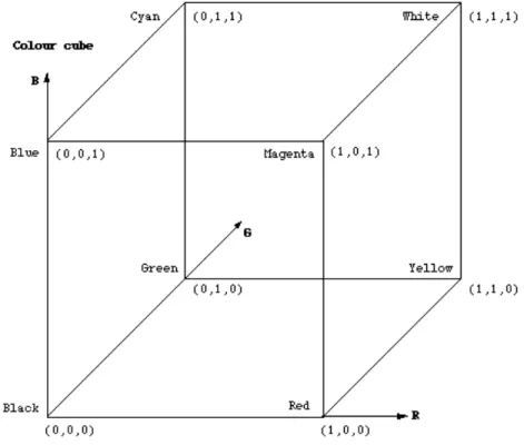
RGB model: This is an additive model that is used by TV monitors and computer screens. Red, Green, and Blue color beams are summed up at the projection screen. All colors that appear on the screen are a summation of R, G, B. To specify each color, the chromaticity values of each of the 3 primary colors need to be specified. R corresponds to the 700nm band of the spectrum, G corresponds to the 546nm band, and B corresponds to the 435nm band. The RGB model is visualized as a unit cube (Figure 1 [4]) where R, G, B are on the X, Y, Z axes.

Figure 1 RGB color model

To form a color, the following linear equations are used [4]: X = 0.490R + 0.310G + 0.200B Y = 0.177R + 0.813G + 0.010B Z = 0.000R + 0.010G + 0.990B

(20)

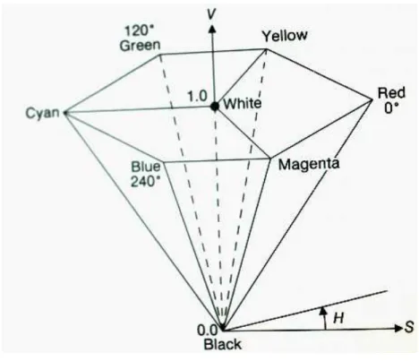
HSV model: While the RGB model is convenient to specify colors in terms of language that hardware/devices would understand, it is difficult for humans to speak in terms of RGB. Humans are more naturally inclined to specify colors in terms of hue, saturation, and intensity. HSI models cater to this need. It is used in computer graphics to specify tints, shades, and tones. Unlike the RGB model, HSI models have cylindrical coordinates. The HSV model (Figure 2 [4]) belongs to the group of HSI models.

Figure 2 HSV model

A point in the RGB coordinate space can be transformed to a point in the HSV coordinate space using the following equations [3]:

V =max (R, G, B) 255

S = max R, G, B − min(R, G, B) max(R, G, B)

(21)

H_@ = cosD@ 1 2 [ R − G + (R − B)] (R − G)G_{+ (R − B)(G − B)} H = H@ ; B ≤ G 360° − H_@; B > G Here, RGB values are in the range 0-255.

The HSV model is used in this project as it aligns with the human representation of color.

2.2 Image features

Image features refer to the information collected from images that can uniquely identify the image or can be used for further processing. Broadly, image features can be classified into general features and domain-specific features [5]. General features, such as color and texture are applicable to all image data and do not depend on the application being considered. Domain-specific features on the other hand, are specific to the application at hand, such as, minutiae in fingerprints. In this work, general features are explored and used in different applications that require image classification.

Based on the locality of features, image features can be categorized into [6]:

(i) Local features: Local features are the patterns in images that differ from its immediate neighborhood. These features are extracted from a patch in the image and are useful in applications such as object recognition. Some examples of local features are Shape Invariant Feature Transform (SIFT), Local Binary Pattern (LBP), and Speeded Up Robust Features (SURF).

(ii) Global features: Global features represent the whole image. These features are extracted considering the whole image as one patch/object and are useful in applications such as image retrieval and image classification, where a rough

(22)

segmentation of objects is available. Some examples of global features are Histogram Oriented Gradient (HOG) and Shape Matrices.

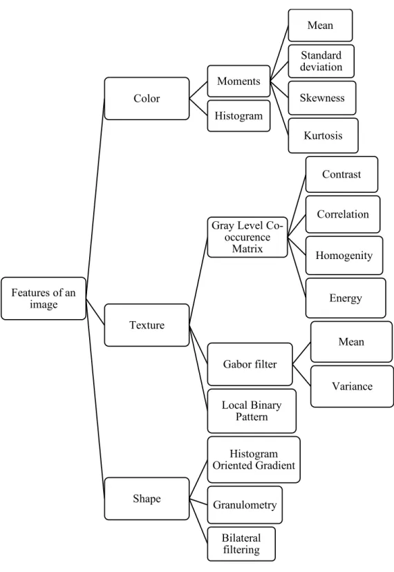
Figure 3 Features of an image Features of an image Color Moments Mean Standard deviation Skewness Kurtosis Histogram Texture

Gray Level Co-occurence Matrix Contrast Correlation Homogenity Energy Gabor filter Mean Variance Local Binary Pattern Shape Histogram Oriented Gradient Granulometry Bilateral filtering

(23)

Based on the visual content of the image, features of images can be categorized into (Figure 3): (i) Color features: Color is the most commonly used image feature that can be recognized

by humans. It is invariant to shape, size, and orientation of the image.

(ii) Texture features: Texture provide information about the color and intensity of the surface in a region of an image. It indicates the roughness or similarity of the region as compared to other regions.

(iii) Shape features: Shapes are yet another feature that can be detected by humans. It represents the contour or outline of object in an image. Ideally, the scale, orientation, and position of objects must not affect the features that are extracted based on shape.

(24)

TABLE I Summary of features extracted Feature Count C ol or Mean of HSV 3 Standard deviation of HSV 3 Skewness of HSV 3 Kurtosis of HSV 3 Histogram - HSV (3x3x5) 45 Te xtu re GLCM - contrast 4 GLCM - correlation 4 GLCM - homogeneity 4 GLCM - Energy 4

Local binary pattern 26

Gabor filter -mean 32

Gabor filter - variance 32

S

h

ap

e

Histogram Oriented Gradients 800

Bilateral Filtering Difference 1

Granulometry 20

984

Figure 4 is a sample image from the category ‘Cartoons’ of the PACS dataset [2] that will be used for demonstrating the various image features:

(25)

Figure 4 Sample image to demonstrate feature extraction

2.2.1 Color features

1. Color moments: Color moments are analogous to central moments and are used to characterize the distribution of colors in an image. They are used to compare the similarity between image. The lower the difference between the color moments of two images, the more similar they are [7] [8].

Consider an image in HSV format with N pixels. Let, pHi be the value of the Hue channel of the ith pixel pSi is the value of the Saturation channel of the ith pixel pVi is the value of the Value channel of the ith pixel

1st moment – Mean: The average of each channel of color in an image.

Mean_O = p_O_Q R ST@ Mean_U = p_U_Q R ST@ Mean_V = p_V_Q R ST@

(26)

2nd moment – Standard Deviation: It is the square root of the variance which is a measure of deviation from the mean.

σ_O= 1 N (pOQ− MeanO)G R ST@ σ_U= 1 N (pUQ− MeanU)G R ST@ σ_V = 1 N (pVQ− MeanV)G R ST@

3rd moment – Skewness: It gives a measure of the shape of the color distribution [8].

sO= 1 N (pOQ− MeanO)Y R ST@ Z s_U = 1 N (pUQ− MeanU)Y R ST@ Z s_V = 1 N (pVQ− MeanV)Y R ST@ Z

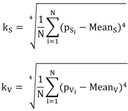
4th_{moment – Kurtosis: It gives a measure of the shape of the distribution in terms of height.}

k_O= 1

N (pOQ− MeanO)\ R

ST@ ]

(27)

k_U= 1 N (pUQ− MeanU)\ R ST@ ] k_V = 1 N (pVQ− MeanV)\ R ST@ ]

Since each moment is computed for each of the 3 channels – H, S, V, there are a total of 12 features that can be extracted from color moments.

TABLE II Color moments of the sample image in Figure 4

H S V

Mean 11.423 23.156 214.397

Standard Deviation 32.053 65.35 75.241

Skewness 2.903 2.883 -1.974

Kurtosis 10.818 13.414 3.579

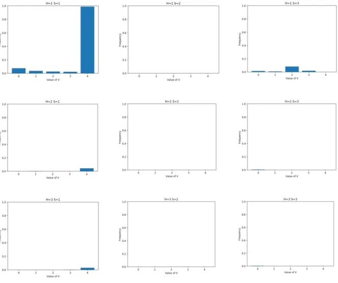
2. Color histogram: A color histogram represents the distribution of colors in an image. It can be visualized either as a distribution of each channel or as a bar chart depicting the number of pixels of a color/channel. Figure 5 represents the 3´3´5 histogram of the image in Figure 4. This set of histograms is generated by creating 3 bins for H channel consisting of 180 values, 3 bins for S channel consisting of 256 values, and 5 bins for V channel consisting of 256 values [4].

(28)

Figure 5 3´3´5 histogram in the HSV color space of the sample image in Figure 4

2.2.2 Texture features

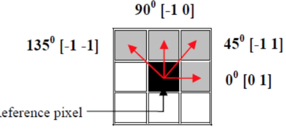
1. Gray Level Co-Occurrence Matrix (GLCM): GLCM was introduced by Haralick for classifying rocks into 6 categories [9]. GLCM is a N´N matrix that is computed for a gray scale image containing N gray levels. The element (i,j) in the GLCM indicates the number of times a pixel of intensity i is adjacent to a pixel of intensity j. Adjacency can be defined in the horizontal, vertical, left diagonal, and right diagonal directions. In terms of angles, these directions translate to 0°, 45°, 90°, and 135° (Figure 6 [10]). 14 statistical features

(29)

Figure 6 GLCM adjacency directions

Out of the 14, four features have been extracted for this project. (i) Contrast: It is a measure of local variations in the GLCM.

Contrast = p_S,a(i − j)G cdedcfD@

S,aTg

(ii) Homogeneity: It measures the distribution of elements when compared to the GLCM diagonal. It is in a sense, the opposite of contrast.

Homogeneity = pS,a

1 + (i − j)G cdedcfD@

S,aTg (iii) Energy: It measures the orderliness of the elements.

Energy = p_S,aG

cdedcfD@ S,aTg

(iv) Correlation: It measures the dependency of elements on its neighbors.

Correlation = p_S,a (i − µS)(j − µa) (σ_SG_)(σ a G₎ cdedcfD@ S,aTg

(30)

TABLE III Haralick features of the sample image in Figure 4 0° 45° 90° 135° Contrast 213.018 311.396 224.946 324.312 Homogeneity 0.71 0.664 0.7 0.669 Energy 0.559 0.551 0.561 0.552 Correlation 0.91 0.869 0.905 0.863

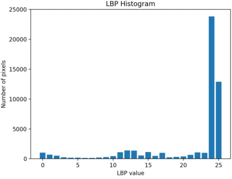
2. Local Binary Pattern (LBP): While GLCM computes global texture features, LBP computes local texture features. Like GLCM, this technique is applied on gray scale images. Considering each pixel as the center, a LBP value is computed and stored in an array that is the same size as the original image. For each center pixel, a radius r is set and n number of points are sampled. If the neighbor selected in the n points has an intensity value less than the center, then it is set to 0, otherwise it is set to 1. Considering all the ones and zeros in a consistent order, the binary number thus formed is converted to decimal. This value then becomes the LBP value of the center pixel. This process is illustrated in Figure 7.

Figure 7 An example of LBP

(31)

Figure 8 LBP histogram of the sample image in Figure 4

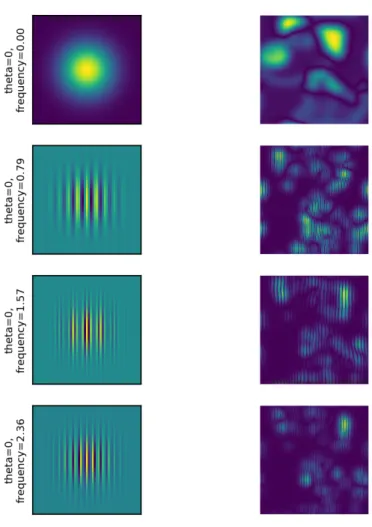
3. Gabor filter: Gabor filters are bandpass filters that are used to extract texture from images. A Gabor kernel of certain size is passed over the image such that it detects edges or textures of given frequency and orientation. A Gabor filter bank is constructed for various combinations of frequency and orientation. The key parameters of this filter are kernel size, sigma (the standard deviation of the Gaussian function), theta (orientation of the normal), lambda (wavelength of the sinusoidal function). Statistical features such as moments of the distribution, median, and entropy can be extracted from the output of the convolution of the image with the Gabor filter. Figure 9 demonstrates the application of a Gabor filter on the sample image in Figure 4.

(32)

Figure 9 Gabor filter applied on the sample image in Figure 4

For this project, 32 9´9 Gabor filters were created, giving 32 mean values and 32 variance values (TABLE IV).

(33)

TABLE IV (Mean, variance) extracted for each Gabor kernel Orientation (in radians) 0 0.39 0.79 1.18 1.57 1.96 2.35 2.75 Frequency (in pixels) 0 78.009, 490.556 77.668, 488.371 74.827, 468.365 77.668, 488.371 78.009, 490.556 77.668, 488.371 74.827, 468.365 77.668, 488.371 0.78 8.119, 1996.668 1.943, 489.464 0.124, 31.533 0.527, 133.487 13.157, 3162.392 0.154, 39.096 0, 0 0.452, 114.631 1.57 1.956, 493.374 0, 0 9.635, 2350.874 0.502, 127.203 2.893, 726.997 0, 0 12.508, 3015.387 0.02, 5.047 2.35 2.462, 619.252 4.785, 1192.217 0.292, 74.367 3.974, 993.435 1.479, 373.866 7.233, 1782.501 0.046, 11.357] 5.718, 1417.57

(34)

2.2.3 Shape features

1. Histogram of Oriented Gradients (HOG): HOG is feature used to detect objects in images. It counts the number of times a gradient orientation occurs in a patch of the image [11]. Plotting the HOG image roughly highlights the outline of the object in the image. The idea behind this feature is that the shape of an object can be represented by its edge direction. The image is split into cells (2´2 patches in this project). Each cell would have pixels within them (16´16 pixels per cell in this project). The horizontal and vertical gradients of the image are then calculated using the Sobel operator. X-gradient highlights vertical edges and Y-gradient highlights horizontal edges. The HOG is computed for every cell. Although HOG is invariant to brightness variations, it is not rotation invariant. The histogram consists of 9 bins representing the angles 0, 20, …, 160. Figure 10 shows an example of how HOG is computed. The HOG computed for each cell is summed up to produce the HOG for the image. Figure 11 shows the HOG image for Figure 4.

(35)

Figure 11 HOG image of the sample image in Figure 4

2. Bilateral filtering: A bilateral filter, when applied on an image, reduces noise and enhances the edges in the image. This is done by replacing a pixel’s intensity with the average intensity of all its neighbors. While this is the functionality of a Gaussian filter, bilateral filter ensures that the edges are preserved [12]. Bilateral filter is useful in differentiating cartoons that have prominent edges from photographs that do not have well-defined edges. A feature that can be extracted from this filter is the mean difference between the original image and the image with bilateral filter applied. The idea is that images like cartoons will have minimal difference while photographs will have a large mean difference [13].

(36)

Figure 12 Bilateral filtering applied to the sample image in Figure 4

3. Granulometry: Granulometry is a method to compute the particle size distribution in an image. To compute the granulometry, a structuring element (SE) and a morphological operation such as dilation or opening is required. An SE is a shape which is scanned over an image to try and capture similar shapes that may be present in the image. Typical shapes for an SE are square, rectangle, and cross. The size of the SE is varied to find objects of a shape based on size. In this project, a disk SE is used as cartoons are more likely to have curved/soft edged objects [4]. Morphological opening is used along with a disk SE in this project. Morphological opening is an operation used to remove noise from images and find specific shapes. Morphological opening is repeatedly applied on the image with different SE sizes, and the granulometry (cardinality of objects of a specific opening size) is recorded. Figure 13 represents the granulometry distribution of the sample image in Figure 4. From the distribution, we can learn that cartoons have lesser number of small sized

(37)

Figure 13 Particle size distribution of the sample image in Figure 4

The pattern spectrum can be derived from the granulometry distribution. It gives an estimate of number of objects of a specific size.

Figure 14: Pattern spectrum of the sample image in Figure 4

(38)

CHAPTER 3 Genetic Algorithms

Evolutionary computation was developed with the idea that it could be used as a tool for optimization and solutions to problems could be evolved using operators of natural selection. Early methods involved representing tasks as finite-state machines and performing mutation by randomly changing the state diagrams. John Holland invented Genetic Algorithms (GA) which was a population-based algorithm. The goal was to study the process of evolution and design a framework that would apply to different applications [14].

A GA is a heuristic search algorithm based on the concepts of natural selection and genetics. The idea is to mimic biological processes such as survival of the fittest, to evolve a solution for a problem. GA is a method of evolving a population of chromosomes to new populations using selection along with operations such as crossover and mutation [14]. Each chromosome consists of genes. Selection operators choose individuals from the population that are the fittest, while crossover and mutation mimic biological processes responsible for introducing diversity to the population. While selection is an exploitation process, crossover and mutation are exploration processes.

Evolutionary algorithms are most suitable for problems that involve a large search space i.e. many possible solutions. Other problems require that new solutions are produced at each stage, to explore new options or they involve complex solutions, that can be processed by hand [14]. GAs, like the process of evolution, depend on the fittest organisms/solutions to survive. The fitness of an organism/solution is determined based on the problem at hand, and it is a factor which continuously evolves. Given this, the parameters of a GA are:

(39)

• a population of individuals/chromosomes – each chromosome is a possible solution to the problem at hand. The population is modified or replaced over n iterations of the algorithm. • fitness function – each chromosome is assigned a fitness value/score which indicates how close the solution represented by the chromosome is, as compared to the expected result. • selection criteria – the fitter the chromosome, the higher the chance it has of being selected. • crossover operator – to create a new chromosome, subsequences of 2 chromosomes are

exchanged at a randomly chosen locus point.

• mutation operator – to create a new chromosome, random bits in the chromosome are flipped.

The procedure of simple genetic algorithm is illustrated in Figure 15 [15]. The parameters of GA used in this project are:

Encoding – binary string (1 represents that the feature has been selected; 0 represents that the feature has not been selected)

Size of population – 50 Number of generations – 100

Crossover operator – 2-point crossover Crossover probability – 0.6

Mutation operator – Bit flip Mutation probability – 0.02 Selection – Roulette Wheel

(40)

Figure 15 Simple GA

Some examples of applications that use GAs, are: optimization tasks, machine learning, economic models, ecological models, immune systems, and social systems [14].

(41)

CHAPTER 4 Feature Selection

In real-world applications, data is collected to the granular level. This has been carried out over many years in the belief that more data means more useful information for processing. With the increase in number of devices worldwide, there has been a surge in the availability of data in a way that storing, handling, and processing data has become difficult. Additionally, the data collected is most often not pre-processed, and hence contains redundant and irrelevant data. Dimensionality reduction techniques have been adopted to reduce the vast dimensions of data to smaller dimensions [16]. The most popular dimensionality reduction techniques combine features to reduce the dimension. Feature selection is one such dimensionality reduction which selects features from the feature set without making modifications to them.

Feature reduction methods have been classified into 3 categories:

i. Filter method: - This method involves ranking features using suitable criteria such

that the highly-ranked features are picked for application [1]. The idea is to filter out lower ranked features. The most important factor in this method is determining the rank or relevance of a feature. A couple of ranking methods are [1]:

a. Correlation criteria: - This is used to detect linear dependencies between features. It is measure using Pearson correlation coefficient.

R i = cov(x*, y) var x_* ∗ var(y)

b. Mutual information: - This measure is used to measure the dependency between features. A value of 0 implies that 2 features are independent.

(42)

The advantages of this method are that it is simple to compute and that it doesn’t rely on learning algorithms. The drawback is that the features selected may not be guaranteed to be non-redundant [1].

ii. Wrapper method: - This method depends on use of classification to determine a feature subset. Exhaustive search methods may be able to arrive at the most optimal result but they can be computationally intensive for large datasets. Therefore, 2 types of wrapper methods may be used [1]:

a. Sequential Search Algorithms: - These algorithms add or remove features until a target optimization function is obtained. Sequential Forward Search algorithm starts with an empty set and adds features as and when they qualify. Sequential Backward Search algorithms start with the entire feature set and progressively eliminate ones that do not meet the performance criteria.

b. Heuristic Search Algorithms: - Genetic algorithms can be used to select features, wherein a chromosome represents the inclusion/exclusion of the set of features. Although this proves to be a convenient method for the selecting features, the main drawback is that the entire model must be built and evaluated for each feature subset considered.

iii. Embedded methods: - This method tries to compensate for the drawbacks of filter and wrapper methods. It involves algorithms that have in-built feature selection methods. This combines the step of selecting features and determining performance into one step [1]. In this project, given that the dataset contains images, the number of features under consideration are so huge that the overhead of building and testing the model for each iteration becomes

(43)

unimportant as compared to selecting a smaller subset of features than originally available. Therefore, GA is used as the method for feature selection.

For feature selection using GA, the most natural and widely used chromosome encoding is the binary string encoding [17, 18, 19, 20, 21, 22, 23]. In this, the chromosome is represented as a bit string in which 1 represents if the feature is selected and 0 otherwise. Some specific implementations used representations which included weighted feature vectors and specific classification model parameters, along with binary string encoding [24, 25]. While the most common crossover and mutation operators are 2-point and random mutation respectively [21, 24], some implementations make use of adaptive crossover and mutation [20, 26], where the probability of crossover and mutation are learnt from iterations. While some implementations used variations of Elitist selection [19, 20, 24, 27] or tournament [18], Roulette wheel seemed to be the most popular selection method [17, 22, 23]. To improve the results, local improvements were used in some cases where low performing features were replaced by high performing features [22]. Fitness functions are application dependent. TABLE V summarizes previous research work done for feature selection using GA.

(44)

TABLE V Summary of GA Parameters used for Feature Selection

Encoding Fitness function Selection Crossover Mutation

Data type

Binary [17, 18, 19, 20, 21, 22, 23]

Information gain [18], similarity measures [18], Standard

deviation, Retrieval precision, Classification accuracy [26], Area under ROC curve [23]

Roulette wheel [17, 22, 23], tournament [18] 2-point [21], m-point [22], adaptive [20, 26], 1- point [23], common feature [18] mutation with probability [17, 18, 23], adaptive [20, 26] Text, image Weighted feature vector + binary encoding + application- specific parameter [24, 25, 28] Classification accuracy [24, 25] Elitist [19, 20, 24, 27] 2-point [24] Change 4 bits [24] Image Random Gauss distribution [27] Text, image

(45)

CHAPTER 5 Classification

An Artificial Intelligence (AI) agent is designed and programmed to make decisions on certain

tasks based on its learning from data. An agent’s learning is essential for the following reasons

[29]:

i. the programmer may not anticipate all possible scenarios

ii. situations may change over time

iii. programmers may not know how to program the agent for a specific situation

Learning can be classified into 2 types based on the order of learning [29]:

i. Inductive learning – learning a rule from specific input-output combinations

ii. Deductive learning – learning a new rule from a general rule.

Learning can also be classified into 2 other types based on the types of feedback [29]:

i. Unsupervised learning – the agent learns without feedback. Example: Clustering

ii. Reinforcement learning – the agent learns from positive or negative feedback from the

previous learning.

iii. Supervised learning – the agent learning from input-output pairs. Example: Classification.

iv. Semi-supervised learning – the agent learns about new unlabeled examples based on data

(46)

5.1 Supervised learning

Given a training set of N (xi, yi) input-output pairs, the task is to learn by searching for a possible

hypotheses (h) that will perform well even on new input-output pairs (Figure 16). The performance

of a hypotheses is measured in terms of accuracy in correctly predicting yj for xj, where (xj, yj)

belong to a test set.

Figure 16 Supervised learning

Classification is a supervised learning problem in which y is a finite set of values. If y can take

only 2 values, then the classification is called binary classification. Regression is a supervised

learning problem in which y is a number.

5.2 Cross-validation

Classifiers need to perform well on previously seen as well as new data. To verify this, validation

is performed on classification models. Validation refers to the process of testing the model using

combinations of training and test data and consolidating the results [30]. Generating different

combinations for validation is a challenging task. Cross-validation is one approach that generates

these combinations by making use of partially seen and unseen data (Figure 17 [30]).

(47)

(i) n-fold cross-validation: Here, the data set is split into n equal parts such that the

percentage of samples of each class is maintained in each fold. The most commonly

used value for n, is 10. In this case, the dataset is split into 10 equal parts. In the first

iteration, the 10th fold is used for testing and the others for training. In the second

iteration, the 9th fold is used for testing and the others for training. The process is

repeated for other folds. Each iteration of validation produces a classification accuracy,

which is then aggregated at the end of the 10 iterations.

(48)

(ii) Leave-one-out cross validation: Suppose there are n entries in the data set, this method

considers n-1 entries for training and the last 1 entry as testing data. The validation

process is repeated n times by leaving one sample out each time for use as test data.

The accuracy is calculated for each iteration and the average accuracy of all iterations

is computed at the end.

(iii) Random sampling: In this method, first, k integers pi (less than n) are randomly

generated. Then, the original data set is shuffled k times to generate k different datasets

Si {i=1,...,k}. Partition each Si into training and validation sets, such that there are pi

samples in the training set and pn-i samples in the validation set.

5.3 Classification models

Given a dataset with 2 or more categories or classes, classification models are mathematical

models that can predict the category of new data based on information from existing data. For

example, let there be 2 classes/categories as depicted in Figure 18.

Figure 18 Two classes - Green and Orange

The task of the classification models is to separate these 2 classes with a clear boundary

differentiating green from orange. Depending on the type of the classification model – linear,

(49)

Figure 19 (a) Linear model (b) Hierarchical model (c) Non-linear model

Support Vector Machine (SVM) – A Linear Model:

This mathematical model makes use of all the data points in the domain and therefore, it is required

that all data are available beforehand. The idea of this model is to place a line (hyperplane)

y = wx%_{+ γ}

in the domain and adjust it in such a way that the classification accuracy is maximized. When there

are multiple classes in the dataset, multiple lines are placed in the domain and adjusted to identify

multiple classes. SVMs may include a kernel when the data is not linearly separable. SVMs also

have the ability to give importance to certain features or sample, thus improving performance.

SVMs are of 2 types:

(i) Linear: The data is expected to be separated by a gap, such that a linear hyperplane can

separate them. The goal is to maximize the distance between the hyperplane and the

nearest data point, which is called margin. Figure 20 (a) is an example of the partition

(50)

Figure 20 (a) Linear SVM (b) Non-linear SVM

(ii) linear: This type of SVM is used when the data cannot be separated linearly.

Non-linear kernels such as homogeneous kernel, non-homogeneous kernel, and Radial Basis

Function kernel, are used. The idea is to find linear separations in higher-dimensional

spaces. Figure 20 (b) is an example of the partition in non-linear SVM.

While SVMs are memory efficient and useful when the data has a large dimension, they are

computationally slow.

Random Forests (RF) – A Hierarchical Model:

RFs are forests of decision trees generated using random sampling, which can be used for both,

classification and regression problems [30]. While decision trees comprise of only one tree for

testing, RFs comprise of multiple decision trees in the testing phase, thus making it a better option

as compared to decision trees. Since, RFs are a group of different decision trees (Figure 21), they

are also called an ensemble method. This method groups together multiple classifiers to form a

strong classifier and improves performance using divide-and-conquer. N samples of data are

(51)

the majority value (in the case of classification). While RFs are fast in execution, they may lead to

data overfitting.

Figure 21 A Random Forest

Neural Networks (NN) – A Non-Linear Model:

Neural networks are models that are designed to mimic the working of the human brain. Multiple

neurons work together to learn new information. Information is stored in the form of weights [31].

It is represented by the equation

Ax = B

where A is the input, B is the outcome, and x are the weights in the network.

The parameters of a neural network are [31]:

(i) Number of neurons

(ii) Number of layers

(iii) Type of connection between neurons

The most basic type of neural network is the perceptron. In its simplest form, the network is

(52)

1 using an activation function, thus performing a binary classification. Learning is done by

adjusting the weights until all the data points in the input dataset are correctly classified. While the

simple single-layer perceptron was effective on linearly separable datasets, the performance was

found to be sub-optimal on non-linear data [31].

The multi-layer feed-forward neural network or multi-layer perceptron (MLP) is the most popular

neural network (Figure 22 [31]). It has input values xi, one or more hidden layers, and an output

layer [31]. While the general architecture of the MLP is like that of the simple perceptron, MLPs

have different activation functions that suit the application at hand. This weights in this type of

network are trained using backpropagation. Higher the weight, the tighter the correlation between

the connection and the outcome.

Figure 22 Multi-layer feed-forward neural network

In this project, all the 3 classifiers have been used to compare their performance for the given

(53)

CHAPTER 6

Experiments and Results

6.1 Applications

While there are numerous applications of image classification, ranging from a simple

differentiation between a cat and a dog, to a more complex application of image spam analysis,

the solution developed in this project focuses on classifying images as photographs or cartoons.

Previous work on classifying images of different domains has primarily focused on classifying

images as computer-generated graphics or camera-captured photographs [32, 33, 34] in the context

of digital forensics and watermarking. An attempt to use GAs to select features for the

classification of images as graphics or photographs, provided positive results in the form of

increased accuracy while reducing the number of features from 234 to 100 [35]. Citing the

complexity of distinguishing between cartoons and photographs, a research on video genre

classification, identified 148 features that could successfully classify cartoons and photographs

[4]. Most image genre classification research make use of either SVMs or neural networks for

classification [4, 32, 33].

6.1.1 Image retrieval

The solution developed in this project focuses on classifying photographs and cartoons to retrieve

images based on a theme/genre. This is particularly useful in the context of a text to picture

conversion system wherein images are retrieved based on information from the text and displayed

in a manner that increases the user’s comprehension [36]. By including the advantages of the

(54)

audience. For example, if the text to picture conversion system is used to convert medical

instructions meant for kids, to illustrations, then the proposed classifier could select only those

images that are cartoons. Figure 23 illustrates how the proposed classification solution could be

utilized to perform a theme-based image retrieval.

Figure 23 Application of the proposed classifier in theme-based image retrieval

6.1.2 Image tampering detection

With the advances made in camera technology, photorealism has become both a boon and a bane.

While making quality photography accessible to the common man and not limiting advanced

features to professional photographers, cameras on devices such as smartphones, along with

various photo-editing software, have led to the increase in image tampering [32]. Images are

tampered with for various reasons ranging from forgery for monetary benefit to reuse without

(55)

manually identify if an image is fake or not [37]. For example, to check if a painting has been

tampered with, experts check the colors of the painting presented, to verify if the colors were

available around the time when the painting was made. As a first pass or filter, image classification

can be used to find out the genuineness of an image by classifying paintings and photographs [37]

[38], and computer generated images and photographs [32, 33, 34]. In this project, we make use

of the features extracted, to distinguish between a piece of art and a photograph.

Given that this project focuses on classifying images into cartoons, photos, and art paintings, the

solution can be trained to classify other domains such as graphics and sketches as well. This is

possible due to the features extracted from the images that cover majority of the feature types of

an image.

6.2 Dataset

The dataset, PACS (Photo, Art Painting, Cartoon, Sketch) [2], used for the experiments in this

project, consists of 9991 images in the 4 domains of photographs, paintings, cartoons, and sketches

(Figure 24 [2]). Images belong to various categories such as ‘dog’, ‘elephant’, ‘giraffe’, ‘guitar’,

‘horse’, ‘house’, ‘person’. Given that the focus of this project is to classify photographs from

cartoons or paintings, only the domains photographs, cartoons and art paintings, consisting of 6062

images, have been used in this project.

Originally, PACS dataset was used to perform domain generalization [2], in which, images from

photograph, painting, and cartoon domains are used for training a model that can then recognize a

(56)

Figure 24 PACS dataset used for domain generalization

6.3 Software used

All experiments were run on a PC with 2.7 GHz Intel Core i5 running MacOS v10.12.6. Source

code was written using Python v2.7.10. The following Python and R (v3.4.3) libraries were used

in the implementation:

Genetic Algorithms - DEAP v1.0.2,

Graph/image plots - matplotlib v2.0.2,

Image feature extraction - scikit-image v0.13.1, OpenCV v3.3.0

Classification algorithms - scikit-learn v0.18.1

(57)

6.4 Results

Binary classification is performed – one for the classification of ‘photo’ vs ‘cartoon’ and another

for the classification of ‘photo’ vs ‘art’.

10-fold cross validation was performed multiple times with different splits, different classification

model and with both, the reduced and the full feature sets. For each combination of data, the

majority over all the iterations is considered as the resultant label. Receiver Operating

Characteristic (ROC) curves are then generated for the reduced and full feature sets with different

classification models. The ROC curves in Figure 25-Figure 30 are representative of one iteration

of 10-fold cross-validation. Average accuracy is computed over multiple iterations of 10-fold

cross-validation, to evaluate the performance of the models.

Case (i): Art vs photo

Training set size: 3346 images – 1503 photos, 1843 art paintings

Validation set size: 372 images – 167 photos, 205 art paintings

Random Forest:

Figure 25 shows the performance of RF for classifying art from photos. The accuracy of

(58)

Figure 25 Art vs Photo: 10-fold ROC curve for RF with Reduced and Full Feature set

SVM:

Figure 26 shows the performance of SVM for classifying art from photos. The accuracy of

classification with SVM is ~75% with the reduced feature set of 492 features and ~58% with the

full feature set.

Figure 26 Art vs Photo: 10-fold ROC curve for SVM with Reduced and Full Feature set

(59)

Figure 27 shows the performance of NN for classifying art from photos. The accuracy of

classification with NN is ~%74 with the reduced feature set of 485 features and ~58% with the

full feature set.

Figure 27 Art vs Photo: 10-fold ROC curve for NN with Reduced and Full Feature set

Case (ii): Cartoon vs photo

Training set size: 3612 images – 2109 cartoons, 1503 photos

Validation set size: 402 images – 235 cartoons, 167 photos

Random Forest:

Figure 28 shows the performance of RF for classifying cartoons from photos. The accuracy of

(60)

Figure 28 Cartoon vs Photo: 10-fold ROC curve for RF with Reduced and Full Feature set

SVM:

Figure 29 shows the performance of SVM for classifying cartoons from photos. The accuracy of

classification with SVM is ~90% with the reduced feature set of 485 features and ~81% with the

full feature set.

Figure 29 Cartoon vs Photo: 10-fold ROC curve for SVM with Reduced and Full Feature set

(61)

Figure 30 shows the performance of NN for classifying cartoons from photos. The accuracy of

classification with NN is ~90% with the reduced feature set of 485 features and ~73% with the full

feature set.

Figure 30 Cartoon vs Photo: 10-fold ROC curve for NN with Reduced and Full Feature set

Figure 31 (a) summarizes the min, mean, and max accuracy of multiple iterations of classifying

art vs photo with various classification models with reduced and full feature set, while Figure 31

(b) summarizes the accuracy of classifying cartoon vs photo.

Figure 31 (a) Accuracy comparison: Art vs Photo (b) Accuracy comparison: Cartoon vs Photo

To confirm that the improvement in accuracy with the reduced feature set is statistically

(62)

which the accuracy results can be replicated. T-tests are used to compare means of two groups and

indicate whether they are different from each other. A T-value trending towards 0, implies that the

groups are similar. A P-value is the probability that the accuracy results occurred by chance. The

lower the P-value, the lesser this chance. P-value 0.05 means that there is 5% chance that the results

occurred by chance. This is also called the 95% confidence interval. TABLE VI summarizes the

results of the T-test comparing the accuracy obtained with different classification models with the

reduced vs full feature set. According to the T-test, there is no statistical difference between the

reduced and full feature set in the case of RF. This can be concluded from the fact that P-value >

0.05 and the confidence interval contains the value 0. Also, this supports the earlier observation

that the accuracies were the same for RF. On the other hand, the difference in accuracies in the

(63)

TABLE VI Comparing accuracies using the T-test

Art-Photo Cartoon-Photo

T-Value P-Value 95% confidence interval T-Value P-Value 95% confidence interval

RF -1.2759 0.205 [-0.0042…0.0009] 1.7453 0.08403 [-0.0001…0.0021]

SVM 5.3012 0.000493 [0.0845…0.2103] 11.211 < 2.2e-16 [0.1072…0.1533]

(64)

CHAPTER 7

Conclusion and Future Work

In this project, we classify cartoons from photos for genre-based image retrieval and classify art paintings from photos to detect image tampering. Since cartoons are better identified using color and shape properties, 878 color and shape features were extracted from each of the 6062 images in the training data set. Along the same lines, since texture of surfaces are more pronounced in art paintings, 106 texture features were extracted. In total, 984 image features were extracted to differentiate between photos, cartoons, and art paintings.

To demonstrate that feature selection not only improves execution time, but also improves classification accuracy, we utilized a GA to select feature subsets from the entire set of features, considering the classifier accuracy as the fitness function. Utilizing this reduced feature set for image classification, the results showed that feature selection improves the accuracy of classification in the case of SVM and Neural Networks, while not making an impact on the classification accuracy in the case of Random Forests. This was expected, as the performance of Random Forests is known to be unaffected by the features selected.

In terms of the appropriateness of the features extracted from the images, the texture-based features helped correctly classify art paintings from the other categories. While color and shape features helped classify cartoons, the classifiers often misclassified cartoon headshots as photos and photos with minimum color variation (such as blue sky) as cartoons.

From our results, we can conclude that GA has a positive impact on the performance of classification, and SVM along with feature selection, performs the best for the classification

(65)

As an extension of this work, we can reuse the solution proposed in this project in other scenarios, such as, to differentiate computer-generated images from camera-generated images, or identify a sketch version of an image from other genres/domains. We can also focus on improving the set of features extracted from images to cater to a wide variety of classification applications. A study comparing GA-based feature selection with other wrapper methods is also planned.

(66)

REFERENCES

[1] G. Chandrashekar and F. Sahin, "A survey on feature selection methods," Computers and Electrical Engineering, vol. 40, no. 1, pp. 16-28, 2014.

[2] D. Li, Y. Yang, Y.-Z. Song and T. Hospedales, "Deeper, Broader and Artier Domain Generalization," in IEEE International Conference on Computer Vision , 2017.

[3] K. N. Plataniotis and A. N. Venetsanopoulos, Color Image Processing and Applications, New York: Springer-Verlag New York, Inc, 2000.

[4] T. I. Ianeva, A. P. de Vries and H. Rohrig, "Detecting cartoons: a case study in automatic video-genre classification," in IEEE International Conference on Multimedia and Expo, 2003.

[5] K. Dittakan, F. Coenen, R. Christley and M. Wardeh, "A Comparative Study of Three Image Representations for Population Estimation Mining Using Remote Sensing Imagery," in Advanced Data Mining and Applications: 9th International Conference, Hangzhou, 2013.

[6] D. A. Lisin, M. A. Mattar, M. B. Blaschko, M. C. Benfield and E. G. Learned-Miller, "Combining Local and Global Image Features for Object Class Recognition," in IEEE Computer Society Conference on Computer Vision and Pattern Recognition, San Diego, CA, 2005.

[7] S. Kodituwakku and S. S, "Comparison of Color Features for Image Retrieval," Indian Journal of Computer Science and Engineering, 2010.

(67)

[8] Wikipedia contributors, "Color moments - Wikipedia," 4 February 2012. [Online]. Available: https://en.wikipedia.org/wiki/Color_moments. [Accessed 28 March 2018]. [9] B. V. Sebastian, U. A and K. Balakrishnan, "Gray Level Co-Occurrence Matrices:

Generalisation and Some New Features," International Journal of Computer Science, Engineering and Information Technology, vol. 2, 2012.

[10] B. Pathak and D. Barooah, "Texture Analysis Based on the Gray-level Co-occurrence Matrix Considering Possible Orientations," International Journal of Advanced Research in Electrical, Electronics and Instrumentation Engineering, vol. 2, no. 9, 2013.

[11] N. Dalal and B. Triggs, "Histograms of oriented gradients for human detection," in IEEE Computer Society Conference on Computer Vision and Pattern Recognition, San Diego, CA, 2005.

[12] S. Paris, P. Kornprobst, J. Tumblin and F. Durand, "A gentle introduction to bilateral filtering and its applications," in ACM SIGGRAPH, New York, 2007.

[13] K. Dade, "Toonify: Cartoon Photo Effect Application," Stanford, CA.

[14] M. Mitchell, An Introduction to Genetic Algorithms, Cambridge, MA: MIT Press, 1998. [15] S. Khuri, Genetic Algorithms, Helsinki, 2017.

[16] J. Leskovec, A. Rajaraman and J. David , "Dimensionality Reduction," in Mining of Massive Datasets, New York, Cambridge University Press, 2014, pp. 415-447.

[17] F. Gómez and A. Quesada, "Genetic algorithms for feature selection in Data Analytics," 01 01 2017. [Online]. Available:

https://www.neuraldesigner.com/blog/genetic_algorithms_for_feature_selection. [Accessed 05 09 2017].

(68)

[18] E. Sivasankar and R. S. Rajesh, "Design and development of efficient feature Selection and classification techniques for Clinical decision support system," Shodhganga, Tirunalveli, 2012.

[19] P. Kushwaha and R. Welekar, "Feature Selection for Image Retrieval based on Genetic Algorithm," International Journal of Interactive Multimedia and Artificial Intelligence, vol. 4, no. 16, pp. 16-21, 2016.

[20] H. Huang, Y. Wu, Y. Chan and C. Lin, "Study on image feature selection: A genetic algorithm approach," in IET International Conference on Frontier Computing. Theory, Technologies and Applications, Taichung, 2010.

[21] C. H. Lin, H. Y. Chen and Y. S. Wu, "Study of image retrieval and classification based on adaptive features using genetic algorithm feature selection," Expert Systems with

Applications, vol. 41, no. 15, pp. 6611-6621, 2014.

[22] I. S. Oh, J. S. Lee and B. R. Moon, "Hybrid genetic algorithms for feature selection," IEEE Transactions on Pattern Analysis and Machine Intelligence, 2004.

[23] B. Sahiner, H. Chan, D. Wei, N. Petrick, M. A. Helvie, D. D. Adler and M. Goodsitt, "Image feature selection by a genetic algorithm: Application to classification of mass and normal breast tissue," Medical Physics, vol. 23, no. 10, pp. 1671-1684, 1996.

[24] J. Lu, T. Zhao and Y. Zhang, "Feature selection based-on genetic algorithm for image annotation," Knowledge-Based Systems, vol. 21, no. 8, pp. 887-891, 2008.

[25] M. L. Raymer, W. F. Punch and E. D. Goodman, "Dimensionality reduction using genetic algorithms," IEEE transactions on evolutionary computation, vol. 4, no. 2, pp. 164-171, 2000.

(69)

[26] L. Liang, J. Peng and B. Yang, "Image Feature Selection Based on Genetic Algorithm," in International Conference on Information Engineering and Applications, Chongqing, 2012. [27] F. Catak, "Genetic Algorithm based Feature Selection in High Dimensional Text Dataset

Classification," WSEAS Transactions on Information Sciences and Application, vol. 12, no. 1, pp. 290-296, 2015.

[28] R. Welikala, M. Fraz, J. Dehmeshki, A. Hoppe, V. Tah, S. Mann, T. Williamson and S. Barman, "Genetic Algorithm Based Feature Selection Combined with Dual Classification for the Automated Detection of Proliferative Diabetic Retinopathy," Computerized Medical Imaging and Graphics, vol. 43, no. 1, pp. 64-77, 2015.

[29] P. Norvig and S. Russell, Artificial Intelligence: A Modern Approach, 3rd Edition ed., Prentice Hall, 2010.

[30] S. Suthaharan, Machine Learning Models and Algorithms for Big Data Classification, Springer International Publishing, 2016.

[31] J. Patterson and A. Gibson, Deep Learning A Practitioner’s Approach, O’Reilly Media, Inc., 2017.

[32] T.-T. Ng and S.-F. Chang, "An online system for classifying computer graphics images from natural photographs," in Security, Steganography, and Watermarking of Multimedia Contents, 2006.

[33] N. Rahmouni, V. Nozick, J. Yamagishi and I. Echizen, "Distinguishing computer graphics from natural images using convolution neural networks," in IEEE Workshop on

(70)

[34] Z. Li, J. Ye and Y. Q. Shi, "Distinguishing computer graphics from photographic images using local binary patterns," in 11th international conference on Digital Forensics and Watermaking, 2012.

[35] W. Chen, Y. Q. Shi, G. Xuan and W. Su, "Computer graphics identification using genetic algorithm," in 19th International Conference on Pattern Recognition, Tampa, 2008. [36] V. Kannan and N. Khuri, "text2collage," March 2018. [Online]. Available:

https://github.com/vandanavk/text2collage.

[37] R. Nemade, A. Nitsure, P. Hirve and S. B. Mane, "Detection of Forgery in Art Paintings using Machine Learning," International Journal of Innovative Research in Science, Engineering and Technology, vol. 6, no. 5, 2017.

[38] F. Cutzu, R. Hammoud and A. Leykin, "Distinguishing paintings from photographs," Computer Vision and Image Understanding, 2005.

[39] M. Everingham, L. Van-Gool, C. Williams, J. Winn and A. Zisserman, "The PASCAL Visual Object Classes Challenge 2007," 2007. [Online]. Available: http://www.pascal-network.org/challenges/VOC/voc2007/workshop/index.html.

[40] A. Aradhya, "Pokemon Images," 2017. [Online]. Available: https://www.kaggle.com/dollarakshay/pokemon-images/data.

[41] A. Mishra, S. Nandan Rai, A. Mishra and C. Jawahar, "IIIT-CFW: A Benchmark Database of Cartoon Faces in the Wild," in 1st Workshop on Visual Analysis and Sketch (ECCVW), 2016.

[42] BagoGames, "New Looney Tunes Movies By X-Men Writers," 28 August 2014. [Online]. Available: https://www.flickr.com/photos/bagogames/15036256406.

(71)

[43] C. Bircanoğlu, "Comic Books Images," 2017. [Online]. Available:

https://www.kaggle.com/cenkbircanoglu/comic-books-classification/data. [44] Wikiart, "Painter by numbers," 2016. [Online]. Available:

(72)

APPENDIX

5 images each (Figure 32-Figure 46), from the categories - photographs, cartoons, and art paintings were retrieved from different sources for testing and the performance of the classification models were evaluated, with the reduced feature set selected by GA. On an average, the GA selects about 485 features out of the 984 features that are extracted for each image. TABLE VII summarizes this performance.

(73)

TABLE VII Performance of the classifiers with the reduced feature set selected by GA

Image True label Classification by RF Classification by SVM Classification by NN

Figure 32 Test Image 1 [39]

Photo Art Photo Photo

(74)

Image True Label Classification by RF Classification by SVM Classification by NN

Photo Art Art Photo

Photo Photo Photo Photo

(75)

Cartoon Cartoon Cartoon Cartoon

Figure 38 Test image 7 [41]