A comprehensible SOM-based scoring system.

Johan Huysmans1_{, Bart Baesens}1,2_{, and Jan Vanthienen}1

1 _{K.U.Leuven, Dept. of Applied Economic Sciences,}

Naamsestraat 69, B-3000 Leuven, Belgium

2 _{School of Management, University of Southampton,}

Southampton, SO17 1BJ, United Kingdom

Abstract. The significant growth of consumer credit has resulted in a wide range of statistical and non-statistical methods for classifying applicants in ‘good’ and ‘bad’ risk categories. Traditionally, (logistic) regression used to be one of the most popular methods for this task, but recently some newer techniques like neural networks and support vector machines have shown excellent classification performance. Self-organizing maps (SOMs) have existed for decades and although they have been used in various application areas, only little research has been done to investigate their appropriateness for credit scoring. In this paper, it is shown how a trained SOM can be used for classification and how the basic SOM-algorithm can be integrated with supervised techniques like the multi-layered perceptron. Classification accuracy of the models is benchmarked with results reported previously.

1

Introduction

One of the key decisions financial institutions have to make is to decide whether or not to grant a loan to a customer. This decision basically boils down to a binary classification problem which aims at distinguishing good payers from bad payers. Until recently, this distinction was made using a judgmental approach by merely inspecting the application form details of the applicant. The credit expert then decided upon the creditworthiness of the applicant, using all possible rele-vant information concerning his sociodemographic status, economic conditions, and intentions. The advent of data storage technology has facilitated financial institutions ability to store all information regarding the characteristics and re-payment behavior of credit applicants electronically. This has motivated the need to automate the credit granting decision by using statistical or machine learning algorithms. Numerous methods have been proposed in the literature to develop credit-risk evaluation models. These models include traditional statistical meth-ods (e.g. logistic regression [13]), classification trees [5], neural network models [1, 4, 18] and support vector machines [2, 15]. While newer approaches, like neu-ral networks and support vector machines, offer high predictive accuracy, it is often difficult to understand the motivation behind their classification decisions. In this paper, the appropriateness of SOMs for credit scoring is investigated. P. Perner and A. Imiya (Eds.): MLDM 2005, LNAI 3587, pp. 80–89, 2005.

c

The powerful visualization possibilities of this neural network model offer a sig-nificant advantage for understanding its decision process. However, the training process of the SOM is unsupervised and initially the predictive power lies there-fore slightly below classification accuracy of several supervised classifiers. In the rest of the paper, we investigate how the SOM can be integrated with super-vised classifiers. Two distinct approaches are adopted. In the first approach, the classification accuracy of individual neurons is improved through the training of a separate supervised classifier for each of these neurons. The second approach is similar to a stacking model. The output of a supervised classifier is used as input to the SOM. Both models are tested on two data sets obtained from a major Benelux financial institution and benchmarked with the results of other classifiers reported in [2].

2

Self Organizing Maps

SOMs were introduced in 1982 by Teuvo Kohonen [10] and have been used in a wide array of applications like the visualization of high-dimensional data [16], clustering of text documents [8], identification of fraudulent insurance claims [3] and many others. An extensive overview of successful applications can be found in [11] and [6]. A SOM is a feedforward neural network consisting of two layers. The neurons from the output layer are usually ordered in a low-dimensional grid. Each unit in the input layer is connected to all neurons in the output layer. Weights are attached to each of these connections. This is similar to a weight vector, with the dimensionality of the input space, being associated with each output neuron. When a training vectorxis presented, the weight vector of each neuron c is compared with x. One commonly opts for the euclidian distance between both vectors as the distance measure. The neuron that lies closest tox is called the ‘winner’ or the Best Matching Unit (BMU). The weight vector of the BMU and its neighbors in the grid are adapted with the following learning rule:

wc=wc+η(t)Λwinner,c(t)(x−wc) (1)

In this expressionη(t) represents the learning rate that decreases during

train-ing.Λ_winner,c(t) is the so-called neighborhood function that decreases when the

distance in the grid between neuron c and the winner unit becomes larger. Often a gaussian function centered around the winner unit is used as the neighborhood function with a decreasing radius during training. The decreasing learning rate and radius of the neighborhood function result in a stable map that does not change substantially after a certain amount of training.

From the learning rule, it can be seen that the neurons will move towards the input vector and that the magnitude of the update is determined by the neighborhood function. Because units that are close to each other in the grid, will receive similar updates, the weights of these neurons will resemble each other and the neurons will be activated by similar input patterns. The winner units for similar input vectors are mostly close to each other and self-organizing maps are therefore often called topology-preserving maps.

3

Related Research

In [12], a model based on self-organizing maps is used to predict corporate bankruptcy. A data set containing 129 observations and 4 variables was divided into a training and a test data set with the proportion between bankrupt and solvent companies being almost equal. A 12 by 12 map was trained and divided into a zone of bankruptcy and a zone of solvency. This division of the map was obtained by labelling each neuron with the label of the most similar training example. Unseen test observations were classified by calculating the distance be-tween the neurons of the map and the observations. If the most-active neurons were in the solvent zone, the observation was classified as good. It is concluded that the percentage correctly classified observations is comparable with the accu-racy of a linear discriminant analysis and several multi-layered perceptrons. The author’s conclusion is promising for the SOM: the flexibility of this neural model to combine with and to adapt to other structures, wether neural or otherwise, augurs a bright future for this type of model.

In [9], several SOM-based models for predicting bankruptcies are evaluated. The first of the models, SOM-1, is very similar to the model described above, but instead of assigning each neuron the label of the most similar observation, a voting scheme is used. For each neuron of the map, the probability of bankruptcy is estimated as the number of bankrupt companies projected onto that node divided by the total number of companies projected on that neuron. A second, more complex model was also proposed (SOM-2). It consists of a small variation to the Basic SOM-algorithm as explained above. Each input vector consists of two types of variables: the financial indicators and the bankruptcy indicators. Only the financial indicators are used when searching which unit is the BMU. Afterwards, the weights are updated with the traditional learning rule from equation 1. These weight updates are not only made for the financial indicators but also for the bankruptcy indicators. The weight of the bankruptcy indicator after training is used as an estimate for the conditional probability of bankruptcy given the neuron. Compared to other classifiers, like LDA and LVQ, SOM-1 was clearly outperformed. SOM-2 performed much better and more importantly: its classification accuracy was quite insensitive to the map grid size.

4

Description and Preprocessing of the Data

For this application, two different data sets were at our disposal. The charac-teristics of these data sets are summarized in Table 1. The same data sets are described in detail in a benchmarking study of different classification algorithms [2]. In this benchmarking study, two thirds of the data were used for training and one third as test set. The same training and test sets will be used in this paper. Additional measures like sensitivity and specificity for these classifiers are also given in Table 1. Sensitivity measures the number of good risks that are correctly identified while specificity measures the number of bad risks that are correctly classified.

Table 1.Description of the Datasets

name Bene1 Bene2

number of obs. 3123 7190

number of variables 27 27

good/bad 67:33 70:30

best classifier RBF LS-SVM(73.1%) MLP(75.1%)

sens/spec 83.9%/52.6% 86.7%/48.1%

Both data sets contain several categorical variables, likegoal of the loan and residential status. A weights of evidence encoding [14] was performed to trans-form them into numerical variables. After pertrans-forming the weights of evidence encoding for the categorical variables, an additional normalization was done for all variables.

5

Exploratory Data Analysis

SOMs have mainly been used for exploratory data analysis and clustering. In this section, the basic SOM-algorithm will be applied to the Bene1 data set. A map of 6 by 4 neurons is used because it is small enough to be conveniently visualized. All analyzes are performed with the SOM-toolbox for Matlab [7].

To examine if ‘good’ and ‘bad’ risk observations are projected onto different units, we can calculate for each observation the winner neuron. For the Bene1 data set, this results in Figure 1(a). In each neuron, the number of good and bad risk observations that were projected onto that neuron, are given. For example,

g(122) b(97) g(6) b(4) g(81) b(23) g(73) b(7) g(14) b(1) g(174) b(13) g(51) b(40) g(36) b(13) g(50) b(19) g(77) b(9) g(7) b(2) g(46) b(13) b(131) g(92) b(29) g(20) g(22) b(16) g(45) b(6) g(52) b(2) g(25) b(2) b(91) g(48) b(54) g(33) g(97) b(31) g(109) b(50) g(46) b(10) g(74) b(19) (a) Number of hits per neuron for training data

(b) Number of hits per neuron. (Dark Gray Bars indicate Good risks; Light Gray Bars represent Bad Risks)

the upper-left neuron was the BMU for 219 training observations, from which 122 were good and 97 were bad. The same information is also given in the left part of Figure 1(b). In this figure, the size of the bar indicates the number of good and bad observations projected onto each neuron. Notice that the scale of the bars is different for ‘good’ and ‘bad’ risk categories. The right part of Figure 1(b) contains the same information, but this time for the unseen test data. From the graphs, it can be noticed that bad risks tend to be projected onto the neurons in the upper half of the grid, but that the SOM is not able to achieve a clear separation. This corresponds with the results from [2], even powerful techniques like Support Vector Machines are not able to obtain a very high degree of accuracy on the Bene1 data set.

6

Classification

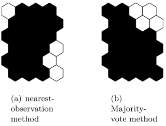
The SOM we created can also be used for classification. In [12], a SOM is created and each neuron is assigned the label of the closest training observation. Pre-dictions for the test data are based on the label of their BMU. Using the same labelling on our map of the Bene1 data, results in 4 nodes that are assigned the bad status and 20 nodes a good status. The labelling is shown in Figure 2(a). It can be seen that most of the nodes labelled ‘bad’ are situated in the lower part of the map. From Figure 1(b) however, we know that most bad risk observations are projected on the upper half of the map. The accuracy, specificity and sen-sitivity of this classification method are therefore rather low (respectively 58%, 22% and 76%). Changes in grid size do not considerably alter these results. For the Bene2 data set, with a grid of 6 by 4, accuracy, specificity and sensitivity are respectively 66%, 14% and 88%. These numbers are considerably below the per-formance of several supervised classifiers reported in [2]. Instead of using only the closest training observation for labelling each neuron, more sophisticated techniques, like k-nearest neighbor, might prove useful.

(a) nearest-observation method (b) Majority-vote method

Fig. 2.Classification of neurons (White: nodes assigned Bad status, Black: nodes as-signed Good Status

0.4 0.5 0.6 0.7 0.8 0.9 1

Fig. 3.Accuracy in each node for Majority-vote method (Bene1 Test Data)

A second way of labelling the neurons was proposed in [9]: each node receives the label of the class from which most training observations are projected on the node. This method will always result in a greater classification accuracy on the training data. Figure 2(b) shows this labelling for the Bene1 data with a 6 by 4 grid. The accuracy, specificity and sensitivity of this map are respectively 71.0%, 44.57% and 84.9%. For the Bene2 data, with the same map size, classification performance was 69.7% because the model assigns the ‘good’ label to all-but-one neuron and will therefore mainly just predict the majority class.

However, it is more interesting to identify the neurons of the map that are responsible for most misclassifications. Figure 3 gives an overview of the clas-sification accuracy in each node for the Bene1 data. Dark nodes are neurons with low classification accuracy. The size of the neurons is an indicator of the number of observations for which that neuron is the BMU. We can see that some neurons are the BMU for lots of observations, while others are the BMU for only a few examples. The presence of large and dark neurons in Figure 3 will indicate a bad classification accuracy of the map. For the Bene1 data set, it can be seen that the lower part of the map has a good classification accuracy. The upper half of the grid shows worse accuracy. For some nodes, the accuracy is below 50%. Fortunately, only few observations are projected onto these nodes. From the figure, we conclude that many observations are pro-jected onto the first neuron of the top row and that not all of these observa-tions belong to the category ‘good’, because classification accuracy is low. In the following section, a more detailed model is elaborated. Observations that are projected onto neurons with low accuracy, will not receive the standard labelling of these nodes, but will instead be classified by independent mod-els. If a SOM is used as new model, a hierarchy of SOMs for prediction is obtained.

7

Integration of SOMs with Other Classification

Techniques

In the previous sections, we have shown that SOMs offer excellent visualiza-tion possibilities that leads to a clear understanding of the decisions made by

these models. But due to their unsupervised nature, SOMs seem not able to obtain the degree of accuracy achievable by several supervised techniques, like multi-layer perceptrons or support vector machines. In this part, the classifi-cation performance of the SOMs will be improved by integrating them with these supervised algorithms. There are two possible approaches for obtaining this integration. One possibility is to first train a SOM and then use the other classification techniques to improve the decisions made by the individual neu-rons of this SOM. A second possibility is to use the predictions of the supervised classifiers as inputs of the SOM. These two approaches are now discussed in more detail.

7.1 Improving the Accuracy of Neurons with Bad Predictive Power

From Figure 3, we can observe that not all neurons achieve the same level of accuracy when predicting the risk category of an applicant. The lack of accu-racy of the predictions made by the neurons in the top rows is compensated by the almost perfect predictions in the lower half of the map. A two-layered approach is suggested in this section. For neurons that achieve almost perfect accuracy on the training data when using one of the models from the previ-ous section, nothing changes. All the observations projected on one of these neurons, will therefore receive the same label. There are only changes for neu-rons whose level of accuracy on the training data lies below a user-specified threshold. For each of these neurons, we build a classifier based on the train-ing examples projected on that neuron. In our experiments, we used feedfor-ward neural networks as classifiers for each of the neurons, but there is no necessity for the classifiers being of the same type. The user-specified accu-racy threshold was fixed at 58% for the Bene1 data set with a 6 by 4 map. This value has been estimated by a trial-and-error procedure. A threshold that is set too low will give no improvement over the above mentioned classifiers because no new models will be estimated. The opposite, a very high thresh-old, will result in too many new classifiers to be trained. With a threshold of 58%, three models will be trained: two for the first two neurons of the top row and one for the third neuron of the third row. We tested with sev-eral different values for the number of hidden neurons in the neural networks. The simplest case, with only one hidden neuron delivered best results with an accuracy on the test set of 71.3% averaged over 100 independent trials. This is almost no improvement over the majority vote classifier that showed an accuracy of 71.0%. It seems that the increase in accuracy of the 3 newly trained classifiers is only marginal. For some neurons, a decrease in the per-centage correctly classified can even be noted. It seems extremely difficult to separate the applicants that are projected on these neurons. A possible im-provement might result from requesting additional information if an applicant is projected on one of the low-accuracy neurons and then training the feed-forward neural networks with this additional information. For applicants that are projected on one of the other neurons, requesting this additional

informa-tion is not necessary. The results for Bene2 are similar. A threshold of 65% results in 9 additional classifiers to be trained of which most are situated in the upper half of the map. The accuracy, averaged over 100 independent trials, improves to 71.9% compared with the original performance of the majority-vote method of 69.7%. Specificity and sensitivity are respectively 26.8% and 91.1%.

7.2 Stacking Model

A stacking model [17] consists of one meta-learner that combines the results of several base learners to make its predictions. In this section, a SOM will be used as the meta-learner . The main difference with the previous section is that the classifiers are trained before training the SOM and not afterwards. The classifiers also learn from all available training observations and not from a small subpart of it.

In our experiments, we start with only one base learner, a multi-layer percep-tron with 2 hidden neurons, which achieves an average classification accuracy of 72.5% on the Bene1 data set (75.1% on Bene2). The input of the meta-learner, the SOM, consists of the training data augmented with the output of this MLP. A small variation to the above described basic SOM-algorithm is used. Instead of finding the BMU by calculating the euclidian distance between each neuron and the sample observation, a weighting factor is introduced for each variable. Heavily weighted variables, in our case the output from the MLP, will contribute more during formation of the map. The distance measure, with n the number of variables, can be written as:

x−wc=

n

i=1

weight_i|x_i−w_c,i|2 ₍₂₎

The update rule from equation 1 does not change. So introducing the weights only affects finding the BMU’s of the SOM [7].

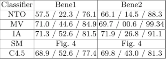
Table 2.Overview of Classification Results (accuracy, specificity and sensitivity)

Classifier Bene1 Bene2

NTO 57.5 / 22.3 / 76.1 66.1 / 14.5 / 88.3 MV 71.0 / 44.6 / 84.9 69.7 / 00.6 / 99.34

IA 71.3 / 52.6 / 81.5 71.9 / 26.8 / 91.1

SM Fig. 4 Fig. 4

C4.5 68.9 / 52.6 / 77.4 69.8 / 43.0 / 81.3

NTO=‘Nearest Training Observation’-method, MV= ‘Majority vote’-method, IA= Improving Accuracy of Neurons with bad Predictive Power, SM= Stacking Model

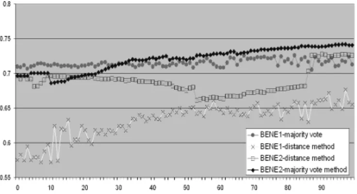
For the experimental study, all the weighting factors of the original variables were fixed at a value of one while the weighting factor of the MLP-input was varied between 1 and 100. Classifications were made by both methods discussed above: the majority-vote method and the nearest-distance method. Figure 4 gives an overview of the classification accuracy for each method and for both data sets with a grid size of 6 by 4.

It can be seen that performance of the nearest-distance method is always below the performance of the majority-vote method. Second, we conclude that the weighting factor of the MLP plays a crucial role in the classification per-formance of the integrated SOM. In general, the larger the weighting factor is, the more the output of the integrated SOM resembles the output of the MLP. There is however a large amount of variance present in the results. A small change in weighting factor can significantly change the performance observed.

In theory, the stacking model can be used in combination with the previous method of integration, but the degree of complexity of the resulting model is high and the advantage of the SOM’s explanatory power is lost. This approach was therefore not analyzed in greater detail.

8

Conclusion

In this paper, the appropriateness of self organizing maps for credit scoring has been investigated. It can be concluded that integration of a SOM with a super-vised classifier is feasible and that the percentage correctly classified applicants of these integrated networks is higher than what can be obtained by employing solely a SOM. The first method, which trains additional classifiers for neurons with bad predictive power withstands competition of other white-box techniques like C4.5. Several topics are still open for future research. For instance, we did not investigate in detail what the influence of the map size is on the results. A combination of SOMs with several different types of supervised classifiers was also not tested. Comparison of the component planes of these different classifiers might visually show where the predictions of the models agree and where they disagree.

References

1. A. Atiya. Bankruptcy prediction for credit risk using neural networks: A survey and new results. IEEE Transactions on Neural Networks, 12(4):929–935, 2001. 2. B. Baesens, T. Van Gestel, S. Viaene, M. Stepanova, J. Suykens, and J. Vanthienen.

Benchmarking state of the art classification algorithms for credit scoring.Journal of the Operational Research Society, 54(6):627–635, 2003.

3. P. Brockett, X. Xia, and R. Derrig. Using kohonen’s self-organizing feature map to uncover automobile bodily injury claims fraud. International Journal of Risk and Insurance, 65:245–274, 1998.

4. M.-C. Chen and S.-H. Huang. Credit scoring and rejected instances reassigning through evolutionary computation techniques. Expert Systems with Applications, 24:433–441, 2003.

5. R. Davis, D. Edelman, and A. Gammerman. Machine learning algorithms for credit scoring applications.IMA Journal of Mathematics Applied in Business and Industry, 4:43–51, 1992.

6. G. Deboeck and T. Kohonen. Visual Explorations in Finance with selforganizing maps. Springer-Verlag, 1998.

7. Helsinki University of Technology. Som toolbox for matlab, 2003.

8. T. Honkela, S. Kaski, K. Lagus, and T. Kohonen. WEBSOM—self-organizing maps of document collections. In Proceedings of WSOM’97, Workshop on Self-Organizing Maps, Espoo, Finland, June 4-6, pages 310–315. Helsinki University of Technology, Neural Networks Research Centre, Espoo, Finland, 1997.

9. K. Kiviluoto. Predicting bankruptcies with the self-organizing map. Neurocom-puting, 21:191–201, 1998.

10. T. Kohonen. Self-organized formation of topologically correct feature maps. Bio-logical Cybernetics, 43:59–69, 1982.

11. T. Kohonen. Self-Organising Maps. Springer-Verlag, 1995.

12. C. Serrano-Cinca. Self organizing neural networks for financial diagnosis.Decision Support Systems, 17:227–238, 1996.

13. A. Steenackers and M. Goovaerts. A credit scoring model for personal loans.

Insurance: Mathematics and Economics, 8(1):31–34, 1989.

14. L. Thomas. A survey of credit and behavioural scoring; forecasting financial risk of lending to consumers. International Journal of Forecasting, 16:149–172, 2000. 15. T. Van Gestel, B. Baesens, J. Garcia, and P. Van Dijcke. A support vector machine

approach to credit scoring. Bank en Financiewezen, 2:73–82, 2003.

16. J. Vesanto. Som-based data visualization methods. Intelligent-Data-Analysis, 3:111–26, 1999.

17. D. Wolpert. Stacked generalization. Neural Networks, 5:241–259, 1991.

18. M. Yobas and J. Crook. Credit scoring using neural and evolutionary techniques.

IMA Statistics in Finance, Journal of Mathematics Applied in Business and In-dustry, 11:111–125, 2000.