The University of Melbourne
Autoregressive Generative Models
and
Multi-Task Learning
with
Convolutional Neural Networks
Florin Schimbinschi
Submitted in total fulfilment of the requirements
of the degree of Doctor of Philosophy
At a high level, sequence modelling problems are of the form where the model aims to predict the next element of a sequence based on neighbouring items. Common types of applications include time-series forecasting, language mod-elling, machine translation and more recently, adversarial learning. One main characteristic of such models is that they assume that there is an underlying learnable structure behind the data generation process, such as it is for lan-guage. Therefore, the models used have to go beyond traditional linear or dis-crete hidden state models.
Convolutional Neural Networks (CNNs) are the de facto state of the art in computer vision. Conversely, for sequence modelling and multi-task learn-ing (MTL) problems, the most common choice are Recurrent Neural Networks (RNNs). In this thesis I show that causal CNNs can be successfully and effi-ciently used for a broad range of sequence modelling and multi-task learning problems. This is supported by applying CNNs to two very different domains, which highlight their flexibility and performance: 1) traffic forecasting in the context of highly dynamic road conditions - with non-stationary data and nor-mal granularity (sampling rate) and a high spatial volume of related tasks; 2) learning musical instrument synthesisers - with stationary data and a very high granularity (high sampling rate - raw waveforms) and thus a high temporal volume, and conditional side information.
In the first case, the challenge is to leverage the complex interactions be-tween tasks while keeping the streaming (online) forecasting process tractable and robust to faults and changes (adding or removing tasks). In the second case, the problem is highly related to language modelling, although much more difficult since, unlike words, multiple musical notes can be played at the same
time, therefore making the task much more challenging.
With the ascent of the Internet of Things (IoT) and Big Data becoming more common, new challenges arise. The four V‘s of Big Data (Volume, Velocity, Va-riety and Veracity) are studied in the context of multi-task learning for spatio-temporal (ST) prediction problems. These aspects are studied in the first part of this thesis. Traditionally such problems are addressed with static, non-modular linear models that do not leverage Big Data. I discuss what the four V‘s im-ply for multi-task ST problems and finally show how CNNs can be set up as efficient classifiers for such problems, if the quantization is properly set up for non-stationary data.
While the first part is predominantly data-centric, focused on aspects such as Volume (is it useful?) and Veracity (how to deal with missing data?) the second part of the thesis addresses the Velocity and Variety challenges. I also show that even for prediction problems set up as regression, causal CNNs are still the best performing model as compared to state of the art algorithms such as SVRS and more traditional methods such as ARIMA. I introduce TRU-VAR (Topologically Regularized Universal Vector AutoRegression) which, as I show, is a robust, versatile real-time multi-task forecasting framework which lever-ages domain-specific knowledge (task topology), the Variety (task diversity) and Velocity (online training).
Finally, the last part of this thesis is focused on generative CNN models. The main contribution is the SynthNet architecture which is the first capable of learning musical instrument synthesisers end-to-end. The architecture is de-rived by following a parsimonious approach (reducing complexity) and via an in-depth analysis of the learned representations of the baseline architectures. I show that the 2D projection of each layer gram activations can correspond to resonating frequencies (which gives each musical instrument it‘s timbre). Syn-thNet trains much faster and it’s generation accuracy is much higher than the baselines. The generated waveforms are almost identical to the ground truth. This has implications in other domains where the the goal is to generate data with similar properties as the data generation process (i.e. adversarial exam-ples).
gression) and generative CNN models. The achievements of this thesis are sup-ported by publications which contain an extensive set of experiments and theo-retical foundations.
This is to certify that
1. the thesis comprises only my original work towards the degree of Doctor of Philosophy except where indicated in the Preface,
2. due acknowledgement has been made in the text to all other material used,
3. the thesis is fewer than 80,000 words in length, exclusive of tables, maps, bibliographies and appendices.
Florin Schimbinschi
This thesis has been written at the School of Computing and Information Sys-tems, The University of Melbourne. The major parts of the thesis are Chapters 3, 4 and 5. These are based on published proceeding or submitted papers and I declare that I am the primary author and have contributed> 50% in all of the following:
1. F. Schimbinschi, V.X. Nguyen, J. Bailey, C. Leckie, H. Vu, R. Kotagiri, “Traf-fic forecasting in complex urban networks: Leveraging big data and ma-chine learning” inInternational conference on Big Data, (IEEE BigData) pp. 1019-1024, IEEE, 2015.
2. F. Schimbinschi, L. Moreira-Matias, V.X. Nguyen, J. Bailey, “Topology-regularized universal vector autoregression for traffic forecasting in large urban areas” inExpert Systems with Applications(ESWA) vol. 82, pp. 301-316, Pergamon, 2017.
3. F. Schimbinschi, C. Walder, S.M. Erfani, J. Bailey, “SynthNet: Learning synthesisers end-to-end.” under reviewInternational Conference on Learn-ing Representations, (ICLR) 2019.
First and foremost I would like to thank my family and friends for their support. A very special thanks to Elena - without her encouragement and optimism my PhD experience would have been very different.
I would also like to thank my supervisors, Prof. James Bailey, Dr. Sarah Monazam Erfani and Dr. Xuan Vinh Nguyen for their wisdom and for the expe-rience that I have gained while working as a research student at the University of Melbourne. I would also like to thank all my colleagues and the people that I’ve met in the department throughout this journey.
As a PhD candidate I have also collaborated with people from outside the university, namely Luis Moreira-Matias from NEC Labs Europe and Christian Walder from CSIRO-Data61 Canberra, to whom I am thankful for their research perspective and expertise.
Finally, my research was made possible by CSIRO-Data61 (formerly NICTA). I am thankful for the computational resources that I extensively used, especially in the last part of my candidature.
1 Introduction 3
1.1 Research contributions . . . 7
1.1.1 Outline of contributions . . . 10
2 Background 13 2.1 Autoregressive and sequence models . . . 13
2.1.1 Beyond linear models . . . 16
2.1.2 Feed forward neural networks . . . 17
2.1.3 Convolutional neural networks . . . 20
2.1.4 Autoregressive Generative CNNs . . . 25
2.2 Multi-task learning . . . 31
2.2.1 Regularization for multi-task learning . . . 33
2.2.2 Multi-task learning in neural networks . . . 39
2.3 Model fitting with gradient based methods . . . 41
2.3.1 First order methods . . . 41
2.3.2 Second order methods . . . 45
2.4 Related work . . . 47
2.4.1 Feed forward and convolutional neural networks . . . 47
2.4.2 Multi-task learning . . . 49
2.4.3 Deep generative models . . . 55
3 Peak traffic prediction in complex urban networks 63 3.1 Introduction . . . 63
3.2 Dataset . . . 65
3.3 Exploratory data analysis . . . 65
3.4 Problem setting and related work . . . 69
3.4.1 Spatio-temporal considerations . . . 69
3.4.2 Related research and datasets . . . 70
3.5 Peak traffic volume prediction . . . 72
3.5.1 Initial algorithm selection . . . 72
3.5.2 The effect of increasing window size . . . 73
3.5.3 Exclusive Monday to Friday traffic prediction . . . 74
3.5.4 Augmenting missing data with context average trends . . 75
3.6 Big Data versus Small Data . . . 76
3.6.1 Leveraging the temporal dimension of big data . . . 76
3.6.2 Leveraging Big Data through sensor proximity . . . 77
3.6.3 Performance as a function of location . . . 78
3.7 Discussion and Conclusion . . . 79
4 Topology-regularized universal vector autoregression 81 4.1 Introduction . . . 82
4.2 Related work . . . 86
4.2.1 Traffic prediction methods . . . 87
4.2.2 Topology and spatio-temporal correlations . . . 90
4.3 Topological vector autoregression . . . 95
4.3.1 Topology Regularized Universal Vector Autoregression . . 96
4.3.2 Structural Risk Minimization . . . 98
4.3.3 Regularized Least Squares . . . 99
4.3.4 The function approximator model . . . 100
4.4 An exploratory analysis of traffic data . . . 103
4.4.1 Datasets . . . 103
4.4.2 VicRoads data quality and congestion events . . . 104
4.4.3 Seasonality, Trends, Cycles and Dependencies . . . 105
4.4.4 Autocorrelation profiles . . . 106
4.4.5 Intersection correlations . . . 108
4.4.6 Pair-wise correlations with query station as a function of time . . . 112
4.5.2 Choosing the lag order . . . 114
4.5.3 TRU-VAR vs. Univariate . . . 115
4.5.4 Long-term forecasting: increasing the prediction horizon . 117 4.6 Conclusions and future work . . . 119
5 SynthNet: Learning synthesizers end-to-end 123 5.1 Introduction . . . 124
5.2 Related work . . . 125
5.3 End-to-end synthesizer learning . . . 126
5.3.1 Baseline architectures . . . 127
5.3.2 Gram matrix projections . . . 129
5.3.3 SynthNet architecture . . . 130
5.4 Experiments . . . 132
5.4.1 Audio and midi preprocessing . . . 133
5.4.2 Synthetic registered audio . . . 136
5.4.3 Measuring audio generation quality . . . 137
5.4.4 Hyperparameter selection . . . 139
Global conditioning . . . 142
5.4.5 MOS listening tests . . . 142
5.5 Discussion . . . 143
6 Conclusions 147 6.1 Summary of contributions . . . 147
1.1 VicRoads dataset - 1000+sensors over 6 years of data over a very
broad and dense area. . . 5
1.2 Timbre is given by the overtone series. . . 6
2.1 Converting AR to classic regression via a sliding window. . . 15
2.2 A feed-forward neural network with one hidden layer. . . 18
2.3 DenseNet with a 5-layer dense block with a growth rate of 4. From [78] . . . 19
2.4 A causal convolution with a filter width of 2. The top yellow sig-nal represents the ground truthyvalues and is a shifted version ofx. . . 20
2.5 Dilated convolution with a dilation factor of two. . . 23
2.6 2D Depthwise separable convolution (right) vs. standard (left). . 24
2.7 The dilation block that is repeated every dilation layer, is de-picted inside the dotted line (these are also shown in Figure 2.9). This depicts the operations in each dilated block, and also shows the last two output layers. Adapted from [170]. . . 27
2.8 Left: training an autoregressive model. Right: generation by re-peated sampling. In practice, padding can be added at genera-tion time before the first actual sample is generated. . . 29
2.9 Multiple dilated convolutional layers are stacked. This results in a very large receptive field, which is useful for high bandwidth data such as audio. . . 30
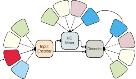
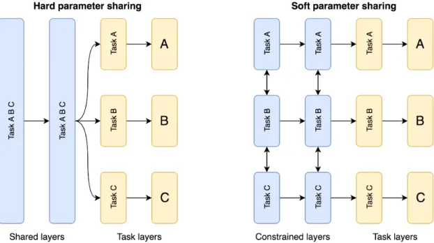
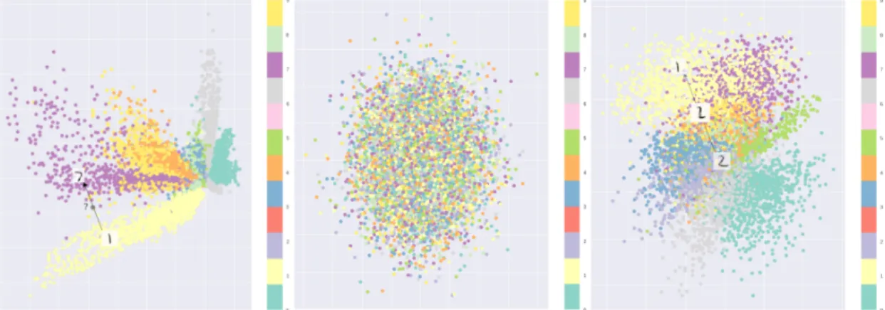
2.10 Multi-task learning with deep neural networks. Shared represen-tations are learned in both the encoder and the autoregressive de-coder. Each colour represents a different modality / task. Taken from [82]. . . 40 2.11 Differences between standard and Nesterov momentum. . . 44 2.12 MTL parameter sharing strategies for neural networks. . . 53 2.13 Left: AE optimized only for reconstruction loss. Middle: VAE
with pure KL loss results in a latent space where encodings are placed near the centre without any similarity information kept. Right: VAE with reconstruction and KL loss results in encodings near the centre that are now clustered according to similarity. . . 59
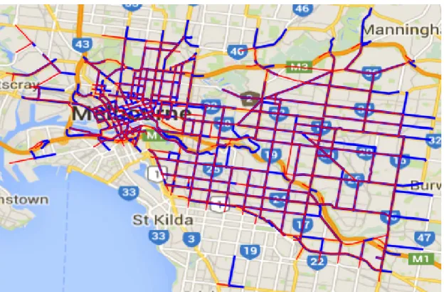
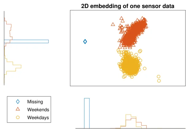
3.1 Melbourne roads with available traffic data are highlighted. Each physical road typically has 2 traffic directions, coloured red and blue. Latitude and longitude coordinates for each sensor are also included. . . 66 3.2 2D embedding of a subset of data for one sensor. Large clusters
are weekdays or weekends. The high density diamond cluster corresponds to days where the traffic volume is zero for an entire day (missing data). . . 67 3.3 92% of sensors have less than 10% missing data, while the rest
can reach up to 56%. There are only 10 sensors without missing data. . . 67 3.4 Average traffic over 6 years accumulated per day of the week. An
outbound road. Evening peak is higher, when commuters depart. 68 3.5 Increasing window size wresults in better accuracy. Results for
∆=20: CNN 93.13, logistic regression 92.83. . . 74 3.6 Weekends are removed. Larger window size∆still results in
bet-ter performance. Top accuracy (93.48, w = 10, CNN) is better than if weekends are included (92.99). . . 75 3.7 Additional data from 3, 5 and 9 closest sensors is added to each
sion). The histogram on the right shows the relative size of each
accuracy cluster. . . 79
4.1 Schematic illustration of the sensor location for both datasets. . . 103
4.2 Sensors above the 95 (black) and 99 (red) quantile after discarding missing data, road sections with many congestion events. . . 104
4.3 Black pixels indicate days with no readings. . . 106
4.4 The daily summary statistics differ for each road segment (Vi-cRoads). . . 107
4.5 Autocorrelation plot for 400 lags. Differencing removes season-ality patterns. Daily seasonseason-ality is clearly observable. . . 107
4.6 Network Wide Autocorrelation Surface. . . 109
4.7 Road sections are marked for either direction (unreliable). . . 110
4.8 Correlation matrix for two different road sections . . . 110
4.9 Ranked road sections by correlation. Query is solid black. The highest ranked are shown in dotted black. There is a large dis-tance between the query and the highest correlated over the en-tire dataset. . . 112
4.10 Sensor 123 correlation at time of day with neighbouring sensors . 113 4.11 RMSE and prediction time as a function of lag (PeMS). . . 115
4.12 Behaviour of error when prediction horizon is increased.µRMSE with solid lines and spread of µ±σ RMSE with dotted lines. Lower is better, error increases linearly with the prediction horizon.118 5.1 Gram matrix projection from Eq. 5.3 Layers in colour, shapes are styles (timbre). . . 129
5.2 SynthNet (also see Table 5.1) with a multi-label cross-entropy loss for binary midi. . . 131
5.3 A signal (dotted line) can be approximated using a lower (left) or higher (right) quantization. Here, the sampling rate (horizontal) is the same in both cases. . . 134
5.4 An 8 bit image is quantized to 1 bit. The process involves first adding noise, before reducing the precision in every pixel. This statistically captures the information in the signal, however at a lower detail fidelity. . . 134 5.5 An abrupt quantization of an audio signal produces correlated
noise patterns (green - right). Dithering implies adding noise (red signal) before the signal is quantized in order to mask the noise. In more advanced cases a noise shaping filter (blue) can be used. 135 5.6 A vintage piano roll used to describe note on-off times. . . 136 5.7 Seven networks are trained, each with a different harmonic style.
Top, losses: training (left) validation (right). Bottom, RMSE-CQT: DeepVoice (left [Tbl. 5.3, col. 6]) and SynthNet (right [Tbl. 5.3, col. 8]). DeepVoice overfits for Glockenspiel (top right, dotted line). Convergence rate is measured via the RMSE-CQT, not the losses. The capacity of DeepVoice is larger, so the losses are steeper.
. . . 138 5.8 Left: 1 second of ground truth audio of Bach’s BWV1007 Prelude,
played with FluidSynth preset 56 Trumpet. Center: SynthNet high quality generated. Right: DeepVoice low quality generated showing delay. Further comparisons over other instrument pre-sets are provided in Figure 5.9. I encourage the readers to listen to the samples here: http://bit.ly/synthnet_appendix_a . . . 138 5.9 Audio samples and visualizations here:http://bit.ly/synthnet_
appendix_a . . . 144 5.10 Gram matrices extracted during training, every 20 epochs. Top
left: extracted from Equation 5.3. Top right: extracted from Equa-tion 5.2. Bottom left: extracted from the filter part of EquaEqua-tion 5.2. Bottom right: extracted from the gate part of Equation 5.2. . . 145
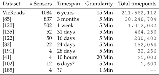
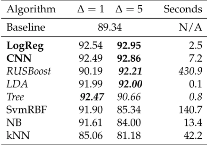
3.1 Comparison of the VicRoads dataset with ones from literature. . . 69 3.2 Network wide classification accuracy and average running time
on a random subset (15%) of sensors. One independent predictor per sensor. . . 73 3.3 Adding mean trend values for missing data increases accuracy. . 75 3.4 Big Data is relevant on the temporal dimension: accuracy
de-creases as the variety and volume of the full dataset is reduced. . 77
4.1 Comparison of TRU-VAR properties with state of the art traffic forecasting methods. Properties that couldn’t be clearly defined as either present or absent were marked with ‘∼’. . . 85 4.2 VicRoads dataset - Average RMSE Topology regularized
uni-versal vector autoregression (TRU-VAR) outperforms univariate models for all f except SVR-L1. . . 115
4.3 VicRoads dataset - Average MAPE Topology regularized uni-versal vector autoregression (TRU-VAR) outperforms univariate models for all f except SVR-L1. . . 116
4.4 PeMS dataset - Average RMSETopology regularized universal vector autoregression (TRU-VAR) outperforms univariate mod-els for all f except LLS-L1. . . 116
4.5 PeMSdataset - Average MAPE Topology regularized universal vector autoregression (TRU-VAR) outperforms univariate mod-els for all f except LLS-L1. . . 117
5.1 Differences between the two baseline architectures and SynthNet. 128
5.2 Three setups for filter, dilation and number of blocks resulting in a similar receptive field. . . 140 5.3 Mean RMSE-CQT and 95% confidence intervals (CIs). Two
base-lines are benchmarked for three sets of model hyperparameter settings (Table 5.2), all other parameters identical. One second of audio is generated every 20 epochs (over 200 epochs) and the error versus the target audio is measured and averaged over the epochs, per instrument. Total number of parameters and train-ing time are also given. All waveforms and plots available here:
http://bit.ly/synthnet_table3 . . . 141 5.4 RMSE-CQT Mean and 95% CIs. All networks learn 7 harmonic
styles simultaneously. . . 142 5.5 Listening MOS and 95% CIs. 5 seconds of audio are generated
from 3 musical pieces (Bach‘s BWV 1007, 1008 and 1009), over 7 instruments for the best found models. Subjects are asked to listen to the ground truth reference, then rate samples from all 3 algorithms simultaneously. 20 ratings are collected for each file. Audio and plots here:http://bit.ly/synthnet_mostest . . . 143
Chapter 1
Introduction
The massive amount of data that is being collected from today’s devices is tremendous. This fuels the need for ever more efficient and easily deployable algorithms. Sequence modelling and multi-task learning (MTL) problems are ubiquitous. In the current information age, connectivity is a core design com-ponent of any physical device, enabling the control and exchange of data. Cur-rently, there are many networks of physical devices such as home appliances, cars, wind farms, and in general virtually any sort of device that has embedded networking electronic components. The network of such connected devices has come to be known as the Internet of Things (IoT). Consequently, there is an abundance of time series data that can be collected from such networks (Big Data).
Traditionally, recurrent neural networks (RNNs) have been the go-to gener-ative method for sequential data. Although CNNs are practically ubiquitous in computer vision problems, their full potential has not yet been explored for generative models and multi-task learning. In this thesis I show that CNNs can be not only highly efficient and accurate but also versatile to deploy and can be applied to a broad range of problems, from detection, forecasting to generative models and also to generating adversarial examples. In subsection 2.1.3 I show that the autoregressive deployment of linear models, Feed Forward Neural Net-works (FFNNs), as well as kernel methods, can also be interpreted as causal convolutional models, exemplified specifically for CNNs. (subsection 2.1.3 also
provides the notation and all the neural network architectural components used throughout this thesis.) Then these are used in a sparsely grouped MTL frame-work applied to forecasting. in Chapter 3 and Chapter 4. Finally, CNNs, MTL and generative models come together in Chapter 5 where SynthNet is intro-duced. This model makes use of several CNN architectural blocks and is trained in a MTL framework with an auxiliary task which improves training.
MTL is essential for applications such as diagnostic (detecting anomalies such as faulty devices), prediction (power output of a wind turbine) and con-trol (best route to take while driving). And yet these are only some of the do-mains where these are central. Any task that involves prediction or control with inter-related time series data can be modelled as a MTL problem. MTL also has applications in optimal control: modeling the kinematics of a robotic arm can be formulated as a multi-task learning problem since the joints (motors) are connected. The latter can also be seen as a sequence to sequence (seq2seq) ap-plication such as language translation. Other examples include fault prediction in computer networks(i.e. anomaly detection) or fraud protection for electronic payments.
Generative models open up many possibilities for IoT. There are many appli-cations including speech synthesis, text analysis and synthesis, semi-supervised learning and model-based control and some are yet to be discovered. Most of these come at a high resolution. The most obvious ones are in natural lan-guage processing, machine translation (and as exemplified before in control problems), text to speech, learning synthesizers, voice cloning, generating au-dio or video based on other data (e.g. translate video speech directly to foreign language based on video lip reading). To connect generative models with IoT and MTL, these can be used to generate artificial or fake data (also known as adversarial examples). This is useful in circumstances when one would like to defend against possible attackers by creating fake sensors or adding fake data in order to confuse attackers. This is useful since, for example DoS attacks are targeted at peak load times.
Many large modern cities have placed sensors under the roads at intersec-tions, in order to record the number of cars that pass through, at one point in time. Then, this data can be used, for example, to control the traffic lights (over
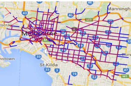
the entire network) and in effect prevent or alleviate congestion. Since there are multiple prediction points that are interdependent, this provides an opportu-nity to study challenging MTL problems in general. The VicRoads dataset (Fig-ure 1.1) was recorded in Melbourne over 5 years. It spans a very large and dense area, is diverse and challenging to tackle since not all sensors were installed at the same time. One other characteristic of this dataset is that approximately half of the sensor stations (tasks) can have more than 50% data missing, which makes the prediction problem more difficult. This dataset is used in Chapter 3 and Chapter 4 to benchmark causal CNNs against other methods such as SVMs, Boosting, Trees, Naive Bayes, K-nearest Neighbours, Linear/Logistic regression and ARIMA.
Figure 1.1:VicRoads dataset - 1000+sensors over 6 years of data over a very broad and dense area.
Although this dataset has a very large number of tasks (1000+) the resolu-tion (granularity) is not very high. Furthermore, it is not clear how to interpret the data generation process. On the other hand, music comes at a high reso-lution (standard commercial quality is at 44.1 thousand frames a second) and music theory and the physics behind the timbre of musical instruments is well understood.
For example, when the note A (110Hz) string is plucked on a guitar, the string vibrates back and forth at many different frequencies at the same. The
lowest is 110 Hz - this is the fundamental frequency (for a timbreless instrument this would be a pure sine wave). Since the string is fixed at both ends, it can only vibrate in multiples of the fundamental frequency: halves are the second harmonic at 220 Hz, thirds are the third harmonic at 330 Hz and so on. This is called the Harmonic series (or the Overtone series) and it is at the basis of how music is structured. What gives an instrument it’s specific timbre, is due to the physics of the instrument (e.g. guitar, trumpet, etc), the materials used and the slight imperfections in the build which are even more subtle. It should also be understood that the overtone series are not necessarily an even multiple of the fundamental frequency.
Figure 1.2:Timbre is given by the overtone series.
However, regardless of the instrument, the fundamental frequency is the same, since that is the musical note that we hear. This brings up the opportu-nity to study MTL and generative models for high resolution time series prob-lems since the content (sequence of notes - fundamental frequencies) can be understood separately from the timbre (overtone series - specific for each mu-sical instrument). Chapter 5 uses synthesized (registered music data) in order to study the learned representations of convolutional autoregressive generative models, trained with an auxiliary MTL task.
1.1. RESEARCH CONTRIBUTIONS
Thesis structure Chapter 2 builds a foundation for better understanding of the proceeding chapters, provides the common notation and a literature review on the existing related work. Chapter 2 is central to all the work in this thesis and especially subsection 2.1.3 which discusses deep causal convolutional neu-ral networks (CNNs). In Chapter 2 I also discuss paneu-rallels among autoregres-sive models and causal CNNs, autoregresautoregres-sive generative models, MTL regular-ization and optimregular-ization methods. I also recommend reading subsection 2.1.4 prior to Chapter 5. Chapter 3 approaches the four V’s of Big Data in the context of multi-task learning with spatio-temporal (ST) prediction problems modelled as classification (peak traffic forecasting). Several methods are benchmarked against causal CNNs.
Chapter 4 builds on top of this work and extends it to continuous outputs (i.e. vector autoregression regression - VAR). In addition, Chapter 4 also dis-cusses scalability and modularity for ST MTL problems where the structure of the graph describing the task relationship is known. Related is section 2.2 in Chapter 2 which provides a detailed theoretical discussion on regularization for MTL and shows that VAR is a special case of MTL.
While Chapters 3 and 4 are dedicated to MTL, Chapter 5 is focused on lan-guage models for music and introduces SynthNet which a WaveNet derived autoregressive generative CNN. Music is a good domain to study the repre-sentations learned by autoregressive CNNs since the structure of instrument harmonics is well known and hence allows the methodical study of learned representations.
1.1
Research contributions
In this thesis I show that CNNs can be very effective and versatile when applied to MTL and generative models. The main advantage is that they are relatively easier to train (vs RNNs) and are faster to train. Despite some architectures having a very large receptive field compared to any other models, they have a very low computational overhead. The large receptive field is critical for high resolution (high sampling rate) signals such as raw audio.
perspec-tive of the four V’s of Big Data (Volume, Variety, Velocity, Veracity). I show that indeed Volume can have a beneficial impact towards performance in the context of MTL for ST problems. I ask the questions whether recent data is more useful on its own and whether Big Data helps even if old data is used. The latter turns out to be true. However, Volume for ST problems specifically, can be the main challenge since the spatial Volume represents the number of tasks. Even with a set of over 1000 such tasks (each with 4 years of data),
I demonstrate in Chapter 3 that causal CNNs outperform other state of the art methods. Velocity is directly linked with the problem setup and modeling when predictions are to be done simultaneously for all tasks (the number of tasks can also change in time). I also show in Chapter 3 that modularity is key to the latter and that causal CNNs can be trained efficiently online (in real-time - Velocity) thus are the best choice in the context of spatio-temporal MTL fore-casting with Big Data. Furthermore, unlike RNNs, these are easy to deploy or redistribute (can be ‘cloned’ easily). The Variety dimension is directly related to task diversity and I show that exchanging data between tasks is indeed benefi-cial. As to the Veracity component, Chapter 4 shows that augmenting missing data with contextual average trends only marginally increases accuracy.
Furthermore, Chapter 4 shows that for this particular MTL problem, de-trending the data is not beneficial since information that the causal CNNs lever-age is removed. Chapter 4 shows that the MTL traffic prediction problem is equivalent to simultaneously solving several sparsely grouped MTL problems. The theoretical framework is benchmarked with state of the art (SOA) models. The results show that causal CNNs outperform other linear and nonlinear mod-els. This is arguably controversial since traditional linear models usually benefit from such methods. This shows that causal CNNs in the context of MTL for ST problems are more versatile and robust towards missing data.
The main contribution of Chapter 4 is the TRU-VAR framework which gen-eralizes MTL for ST problems and shows that solving grouped MTL problems can be equivalent and more efficient to solving a single MTL problem. This chapter also shows that using the topological structure of roads in MTL prob-lems is a better approach towards introducing sparse groups since correlation based methods are not accurate with physical location. Several methods are
1.1. RESEARCH CONTRIBUTIONS
benchmarked within this framework on two different datasets, and for both, the causal CNNs yield the best results.
In conclusion, Chapter 4 shows that TRU-VAR is able to scale well to large datasets, is robust and furthermore is easily deployable with new sensor in-stallations. The adjacency matrix used for generating sparse MTL task groups should be chosen carefully and should be done as a function of the dataset and domain. Furthermore, high resolution data (temporal as well as spatial) is es-sential. Missing data can be an issue and augmenting it does not significantly increase performance, however it should be explicitly marked in order to dis-tinguish it from real events (e.g. congestion in traffic).
The last part of this thesis – Chapter 5 is dedicated to autoregressive genera-tive CNNs. It introduces the SynthNet algorithm which is able to generate high fidelity audio based on only 9 minutes of training data per instrument timbre. While the original algorithm (WaveNet) from which this work was derived was able to generate speech that sounded realistic, the waveforms were very differ-ent to the ground truth. SynthNet is able to generate audio so accurately that the generated waveforms are almost identical to the ground truth. This is very significant since music is more complex than spoken word.
In addition SynthNet trains and converges faster than the baselines since it has fewer parameters. Chapter 5 also gives an explanation of the structure of the learned representations of autoregressive CNNs, which advances the un-derstanding of CNNs for audio closer to the ones in images. This was done by testing the hypothesis that the first causal layer learns fundamental frequencies. This was validated empirically, arriving at the SynthNet architecture.
The method is able to simultaneously learn the characteristic harmonics of a musical instrument (timbre) and a joint embedding between notes and the corresponding fundamental frequencies. This has implications in many fields since the ability to generate signals that match the ground truth with a high fidelity is a very desirable property. Previous methods were not able to do so and were focused purely on the qualitative (how does the audio sound like) measurements while the actual generated data differed from the ground truth.
1.1.1
Outline of contributions
The contributions of Chapter 3 mainly stem from the experiments: (i) modeling prediction as a multi-task learning problem is beneficial;
(ii) the spatio-temporal representation is one of the central issues;
(iii) predicting only on weekdays is easier and separate predictors can be de-ployed separately for weekends or each day of the week;
(iv) adjusting the receptive field size and proximity lowers error;
(v) for classification problems, the quantization of real-valued data is a central issue and should either be avoided or thresholding should be set dynam-ically.
The contributions of Chapter 4 are as follows:
(i) I propose learning Topology-Regularized Universal Vector Autoregres-sion (TRU-VAR), a novel framework that is based on the spatio-temporal dependences between multiple sensor stations;
(ii) The extension of TRU-VAR to CNNs and other nonlinear universal func-tion approximators over the existing state of the art machine learning al-gorithms, resulting in an exhaustive comparison;
(iii) The evaluations performed on two large scale real world datasets, which are different: one is sparse high granularity, the other is dense and has slightly lower granularity;
(iv) Comprehensive coverage of the literature, and an exploratory analysis considering data quality, preprocessing and possible heuristics for choos-ing the topology-designed adjacency matrix (TDAM).
Finally, Chapter 5 makes the following contributions:
(i) I show that musical instrument synthesizers can be learned end-to-end based on raw audio and a binary note representation, with minimal train-ing data;
(ii) Multiple instruments can be learned by a single model;
(iii) I give insights into the representations learned by dilated causal convolu-tional blocks;
1.1. RESEARCH CONTRIBUTIONS
(iv) I propose SynthNet, which provides substantial improvements in quality and training time and convergence rate compared to previous work;
(v) I demonstrate (Figure 5.8) that the generated audio is practically identical to the ground truth;
(vi) The benchmarks against existing architectures contains an extensive set of experiments spanning over three sets of hyperparameters, where I control for receptive field size;
(vii) I show that the RMSE of the Constant-Q Transform (RMSE-CQT) is highly correlated with the subjective listening mean opinion score (MOS);
(viii) I find that reducing quantization error via dithering is a critical prepro-cessing step towards generating the correct melody and learning the cor-rect pitch to fundamental frequency mapping.
Chapter 2
Background
This chapter provides an introduction and an overview of the core topics used throughout the rest of the chapters. In section 2.1 I give an introduction to simple linear models, then I extend the scope to kernel methods and finally discuss Feed Forward Neural Networks (FFNNs). I show that autoregressive models can also be interpreted as causal convolutional models, as exemplified for converting FFNNs to Causal Convolutional Neural Networks (CNNs). sub-section 2.1.4 discusses the WaveNet architecture in detail based on the previous sections. Then, I give an overview of MTL regularization in section 2.2 showing that regularization can be used to share parameters between related tasks and that tasks can be grouped based on a known prior structure. In section 2.3 I discuss gradient based optimization methods for fitting these models. Finally, section 2.4 provides an extensive literature review on autoregressive models, MTL and generative models for time series.
2.1
Autoregressive and sequence models
It is common to model a time series as an autoregressive process. For a time seriesx, each observation xt can be conditioned on the observations at all
pre-vious time stepsx<t ={xt−1,xt−2, . . . ,x1}. The joint probability of a time series
p(x) =
T
∏
t=1
p(xt | x<t) (2.1)
Traditionally, the Autoregressive Moving Average (ARMA) model is used for modelling time series. This stochastic linear model is composed of an Au-toRegressive (AR) and a Moving Average (MA) component. An AR model as-sumes the predicted value to be a linear combination of∆ppast observations:
yt =θ0+ ∆p
∑
i=1
θixt−i+et wheree ∈ N(0,σ) (2.2)
where θ0 is the intercept or bias, yt is the scalar response value, xi are the past
time series observations (or explanatory variables) andet is the random error.
For AR models,∆is known as the order of the model, and is also known as thelag. In the neural network literature∆is referred to as the size of thereceptive field.
While an AR(∆p) model regresses against past values of the time series, a
MA(∆q) model uses the past errors as the explanatory variables (whereµis the
mean of the time series):
yt =µ+
∆q
∑
j=1
φjet−j+et (2.3)
These can be finally combined into the ARMA model:
yt =θ0+et+ ∆p
∑
i=1 θixt−i+ ∆q∑
j=1 φjet−j (2.4)ARMA models, are applied in Chapter 4 and no longer discussed here, for a detailed discussion see [19].
Linear regression For convenience I denote the scalar response value y = xt
and write the vector of explanatory variables as x∆ = (1,xt−1,xt−2, . . . ,xt−∆)
and the parameters θ = (θ0,θ1,θ2, . . . ,θ∆), also including the intercept. Then,
the AR model can be rewritten as classic linear regression:
2.1. AUTOREGRESSIVE AND SEQUENCE MODELS
y= f(x,θ) = θ>x∆ (2.5)
where the total number of observations reduces toN =T−∆.
To lighten the notation and generalize, any autoregressive model f parametrized byθwill be written from now on asy= f(x,θ), as exemplified in Equation 2.5,
which is identical to the AR model described in Equation 2.2. The conversion from an AR process to classic regression is depicted in Figure 2.1 where the grey box represents ∆. The AR process is also described as a causal convolution in Figure 2.4.
Figure 2.1:Converting AR to classic regression via a sliding window.
Logistic regression For regression the goal is to solve problems of the form
f : X →Y ⊆Rwhile for multiclass classification the goal is to find f : X →Y =
{1, 2, . . . ,C} where C is the number of classes. For classification, the softmax function ψ extends linear to logistic regression by representing a probability
distribution overCdifferent possible outcomes:
ψ: RC → ( ψ∈RC | ψi >0, C
∑
i=1 ψi =1 )ψ(xj) = e xj
∑C
c=1exc
∀j ∈ {1, . . . ,C} (2.6)
Then, linear regression becomes a classification problem withCclasses where the following probability is maximized:
P(yi =c | xi;θ) = e (θ>c xi) ∑C j=1e θj>xi (2.7)
Chapter 3 makes use of these models for imbalanced binomial classification as applied to peak traffic forecasting. Chapter 4 later extends this to regression (using the same dataset).
2.1.1
Beyond linear models
The softmax function can be applied in principle to any function approxima-tor f transforming regression to a classification by applying ψ at the outputs.
For multi-class kernel classification methods such as Support Vector Machines (SVMs) the dominating paradigm is to formulate the problem as multiple bi-nary problems where C = 2 and usually extended it as one-vs-rest or all the one-vs-one combinations. However, multi-class extensions exist [103].
Non-linear extensions of linear algorithms can either be done explicitly, or via the kernel trick, which avoids an explicit mapping. To derive a kernelized version of a linear model, I start from the observation that the parameter vector
θcan be expressed as a linear combination of theNtraining samples:
θ=
n
∑
i
αiyixi (2.8)
where αi is the number of times xi was misclassified, also known as the
ex-pansion coefficients.
It can now be clearly seen that the main problem with kernel methods, specifically SVMs is that the complexity lies in the number of examples, and
2.1. AUTOREGRESSIVE AND SEQUENCE MODELS
hence working with large datasets can become problematic. Instead of fitting the parametersθ, the vectorαis updated:
ˆ y= f(θ>x) (2.9) = f N
∑
i αiyixi !> x (2.10) = f N∑
i αiyi(xi·x) (2.11)Finally, the dot product can be replaced with a kernelK. Mercer’s theorem implies that any positive semi-definite matrixK is the Gramian matrix of a set of vectors. A positive semi-definite matrix is a matrixKof dimension N, which satisfies, for all vectorsv, the property:
v>Kv= N
∑
i=1 N∑
j=1 viKijvj ≥0 (2.12)ThenKacts as a feature mapΨwithout computingΨ(x)explicitly, yielding the general kernel method:
f(x,K) =
N
∑
i=1
αiK(xi,x) (2.13)
In practice, however Mercer’s condition can be relaxed for matrices K, still resulting in reasonable performance. For Gaussian processes,Kis also a covari-ance function which implies that the Gram matrixK(i.e. kernel) is a covariance matrix. In this thesis I use Gram matices for visualising the activations of sev-eral layers in Chapter 5.
2.1.2
Feed forward neural networks
Roughly, neural networks can also be thought of as learning kernels, since a nonlinear mapping is learned in a two layer neural network. Indeed, extensions
exist, where (linear) SVMs are used as pure classifiers, based on features learned from neural networks [165, 186]. However, due to the increased computational cost and the lack of availability of multi-class SVMs, this is not often done in practice very often.
Perceptrons The simplest form of neural network is the Perceptron. Even though in the original formulation, the transfer function was the hard sign func-tion, the extension from linear models is trivial and can be done using the logis-tic sigmoid function:
f(x,θ) =σ(θ>x) where σ(x) =1/(1+e−x)
Multi-layer perceptrons Perceptrons can be trivially extended to multi-class problems via the softmax function (Equation 2.6):
h=σ(θ>0x) (2.14)
y= f(x,θ) =ψ(θ>1h) (2.15)
Figure 2.2:A feed-forward neural network with one hidden layer.
Then, the hidden activation hacts as a kernel (but not in a strict definition),
2.1. AUTOREGRESSIVE AND SEQUENCE MODELS
where the representation is learned. This is subsequently passed through a pure linear layer and then passed through the softmax in order to arrive at a multi-class Multi-Layer Perceptron (MLP). The term MLP is a synonym for Feed For-ward Neural Network (FFNN - Figure 2.2) when used for classification. Of course, more than one hidden layer can be used, and this amounts to adding more equations producing multiple hi ∈ {1, . . . ,L} in Equation 2.14 where L
are the number of hidden layers.
Residual connections Most likely residual connections [67] were inspired by Highway Networks [157]. In the latter, an additional weight matrix is used to learn the skip weights. This was simplified. The core idea is to enable short-cuts over layers, by bypassing the non-linear transformation with an identity function. This helps alleviate exploding and vanishing gradients. Adding an additional layer and applying a residual connection over the previous example:
h0 =σ(θ0>x)
h1 =σ(θ1>x) +x
f(x,θ) = ψ(θ>1h1)
In this case,h0will possibly made redundant by skipping the parameters learned
inθ1. Of course, several layers could be skipped at a time. Another extension
of the idea is when residual connections exist from all previous layers to all the next layers. These are referred to as DenseNets [78] (idea shown in Figure 2.3).
2.1.3
Convolutional neural networks
In this section I show that any FFNN dense layer can be converted to a CNN layer. The reverse is also possible but not illustrated here. Firstly, Causal convo-lutions can be obtained by convolving the signal with a shifted version of itself, or by masking future time steps. This process is illustrated in Figure 2.4 and can be examined in relation to Figure 2.1.
Figure 2.4: A causal convolution with a filter width of 2. The top yellow signal repre-sents the ground truthyvalues and is a shifted version ofx.
Discrete convolutions The discrete convolution of two signals f and gis for-mulated as: (f ∗g)[n] = ∞
∑
m=−∞ f [m]g[n−m] = ∞∑
m=−∞ f[n−m]g[m]In the depicted case in Figure 2.4 the parameters θ have support in the set
{θ1,θ2}since the filter width F=2 and therefore a finite summation is used:
f(x,θ) = (x∗θ)[n] =
M
∑
m=−M
x[n−m]θ[m] (2.16)
Feed forward dense layers to convolutional layers Any Feed-Forward Neu-ral Network (dense) layer can be converted to a Convolutional Layer since any
2.1. AUTOREGRESSIVE AND SEQUENCE MODELS
convolution can be constructed as a matrix multiplication. The computations can be constructed using a Toeplitz matrix such asAbelow:
A= a0 a−1 a−2 . . . a−(n−1) a1 a0 a−1 . .. ... a2 a1 . .. ... ... ... .. . . .. ... ... a−1 a−2 .. . . .. a1 a0 a−1 an−1 . . . a2 a1 a0 (2.17)
which is a matrix where Ai,j = Ai+1,j+1 =ai−j.
Then, the convolution operation can be constructed as a matrix multipli-cation where the parameter vectorθ for one layer is converted into a Toeplitz
matrix. For example, the convolution ofθand xcan be written as:
yn = xt = f(x,θ) =θ∗x = θ1 0 . . . 0 0 θ2 θ1 . . . ... ... θ3 θ2 . . . 0 0 .. . θ3 . . . θ1 0 θm−1 ... . . . θ2 θ1 θm θm−1 ... ... θ2 0 θm . . . θm−2 ... 0 0 . . . θm−1 θm−2 .. . ... ... θm θm−1 0 0 0 . . . θm xt−1 xt−2 xt−3 .. . xt−∆ (2.18)
Specifically for the case depicted in Figure 2.4 the Causal convolution is ob-tained by masking x to the observations within the grey box, and referring to the notation in Equation 2.16,m = 2 = F and n = t−∆ = 2. At this point it should be evident that Equation 2.18 is equivalent with Equation 2.5 and can be written compactly as Equation 2.16. In practice, a bias is also commonly used -this is not depicted in Figure 2.4, but one could imagine an extra parameterθ0
which has an input which is always 1.
Prediction horizon While Figure 2.1 and Figure 2.4 depict prediction horizons equal to one, in order to move the prediction horizon further in time, the only necessary change is to shift the yellow depictions to the right in both figures. The prediction horizonh indicates how far in the future predictions are made, in the case of prediction problems.
Output channels It is usually the case that CNNs change the number of input channels. Then, the parameters θc can be repeated as many times as the
num-ber of required output channels Cout is set to. This is equivalent to repeating
the convolution with different learned parameters, as many times as there are output channels. Or another way to imagine the process is to picture several parallel convolutions with the same inputs. Since the learned parameters for each convolution is initialized differently, each will learn a different kernel.
Output observations: Padding & stride An important parameter is the stride, which is labelled only in Figure 2.1. However, Figure 2.4 also depicts a stride of one with the dotted grey box (sliding window). This parameter indicates how many steps to the right the sliding window is moved at one time. For larger strides, the window is moved to the right more than one observation at a time. Padding refers to adding observations (commonly at either the beginning or the end of the time series) in order to change the number of output frames (Equation 2.19. If no padding is used, then the padding is said to bevalidwhile if the output is intended to have the same number of frames as the input, the padding is said to besame.
Dilated convolutions Dilated convolutions are essentially identical with Causal convolutions with the difference that some of the inputs are skipped. Figure 2.5 shows a dilated convolution with a dilation factor of two. Every second input observation is skipped. The convolution is performed as if the skipped input (Figure 2.5 x1 - red) does not exist. However, x1will be used as an input after
the window will be moved to the right for the next operation. Dilated
2.1. AUTOREGRESSIVE AND SEQUENCE MODELS
tions are typically used for high sampling frequency data such as audio, where a large receptive field ∆ is required. Then, multiple such layers as depicted in Figure 2.5 can be stacked on top of each other as it is done in the WaveNet architecture [170].
Figure 2.5:Dilated convolution with a dilation factor of two.
In general the number of output framesToutfor a one dimensional
convolu-tion is given by the following formula:
Tout = Tin
+2×padding−dilation×(filter_width−1)−1
stride +1 (2.19)
Pointwise convolutions Pointwise convolutions, also known as 1x1 convolu-tions or Network in Network are a special case where the filter width is equal to 1 and the only change is the number of output channels. In essence 1x1 convolutions only change the dimensionality of the output. A simpler way to think about depthwise convolutions is to imagine them as a simple feed-forward dense layer where the number of input channels (Figure 2.2 - red) are the number of input neurons and the output channels (Figure 2.2 - blue) are equal to the number of output neurons. This is equivalent to multiplying each observation inxwith a set of parametersθthat change the dimensionality.
Grouped convolutions Convolutions can be grouped. When the number of groups is set to 2 for example, one can think of two separate convolutions being performed in parallel. However each convolution will have access to only half the input channels and will also produce only half the the output channels.
Finally, the outputs will be concatenated to produce the total requested number of channels.
An extreme case of grouped convolutions is when the number of groups is set equal to the number of input channels. In this case, each input channel is convolved with its own set of filters of size Cout/Cin. This case is termed in
literature as a depthwise separable convolution.
A standard convolution filters and combines inputs into a new set of outputs in one single step. In depthwise separable convolutions, each channel is first convolved with its own set of filters, then a 1x1 convolution is applied in order to combine the outputs.
Figure 2.6:2D Depthwise separable convolution (right) vs. standard (left).
In some cases, grouped convolutions happen to work better in practice since filter relationships are sparse. When the number of output channels is large and the kernel size is also large, the computational cost can be significantly reduced. The number of multiplications (or the number of parameters is compared in the equation below, whereCrepresents channels, Wis the width of the kernel and
V is the output volume or the number of output frames:
Standard convolution Depthwise separable conv =
Cin×V×(W+Cout)
Cin×V×W×Cout
= W+Cout
W×Cout (2.20)
It can be seen that when settingW =2 andCout =128, the depthwise
sepa-rable convolution has twice fewer parameters. If the filter width is increased to
2.1. AUTOREGRESSIVE AND SEQUENCE MODELS
W =3 then it will have 66% fewer and so on.
The idea was originally introduced in the AlexNet [97] architecture as an en-gineering feat to speed up training and recently, it has also been applied to low power mobile deep learning vision applications [75]. Parallels to the Inception model [163] have also been made in the Xception model [33] which generalizes the concept. The architectural concept has also proven to be a key component in the MultiModel [82] architecture which consists of a single neural network model that can simultaneously learn multiple tasks from various multiple do-mains.
2.1.4
Autoregressive Generative CNNs
Having discussed most of the ingredients in subsection 2.1.3 here I start by de-tailing the WaveNet architecture. I finally provide a diagram that explains in parallel both the time unrolled view of the architecture, as well as the where the dilated convolutional blocks are located, providing an overall view of the num-ber of frames, channels (dimensions / neurons) and the convolutions. I also explain how the number of frames and the number of channels change between layers. Then I explain the structure of each dilated block in WaveNet and finally put everything together, explaining the skip connections and how to condition the network with other signals.
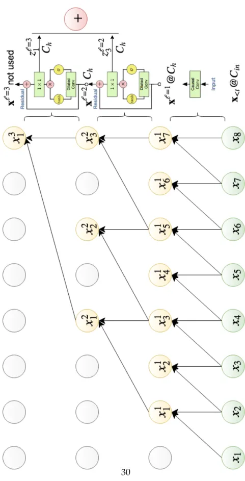
Frames and channels In Figure 2.9 the receptive field∆has 8 frames, consist-ing of{xt−1, . . . ,xt−∆}. This will produce one output ˆxt. In general, for an input
ofT frames, there will beT−∆+1 output frames.
For raw mono audio, the input channels can either be: 1 or 256 if the audio is quantized usingµ-Law companding and then subsequently encoded to a
one-hot 256 valued vector). µ-Law companding only changes the bit depth of the
audio from 216 = 65536 which is standard audio quality to 28 = 256 which reduces the number of possible outputs and makes training possible with the cross-entropy loss.
Dilated convolutions One core ingredient is the dilated convolution. Multi-ple of these are stacked on top of each other, where each layer has a increased dilation rate. In Figure 2.9 I also display the dilated block architecture in order to exemplify how everything in the architecture is put together. This is for a plain architecture without any conditioning.
The first input layer is a convolutional layer with a filter width ofF. In fact all convolutions, except for the output layers have a filter width ofF. The purpose of this layer is to change the number of input channelsCin from whatever the
input dimensionality in x<t is to the number of channels in each dilated block
Ch. In addition, the input layer changes the number of input frames, according
to Equation 2.19 (in Figure 2.9 from 8 to 7).
x1 |{z} Ch =tanh(θin∗ x<t |{z} Cin ) (2.21)
This is followed by a series of dilated block layers (only 2 in Figure 2.7) which all have Ch channels. Every dilation block also changes the number of
frames according to Equation 2.19, reducing them until there is only one frame at the top of the block-layers stacks. This is the main purpose of the dilated blocks - to grow very large receptive fields by stacking dilated convolutions on top of each other, with an ever increasing dilation rate (however the dilation pattern e.g. 1, 2, 4, 8, etc. can be repeated multiple times). There is also no restriction on how the dilation rate increases, it does not necessarily have to be increasing powers of two.
Inside the dilated blocks Each dilated block is composed of two initial con-volutions, side by side, which take exactly the same inputs from the previous layerx`−1. The first one goes through atanh -τactivation while the second one
goes through asigmoid - σ activation. This mechanism is most likely inspired
by recurrent neural networks. In essence, the sigmoid acts like a gating mech-anism that can inhibit the main tanh signal. This is a good approach under the plausible hypothesis that each layer learns coefficients for a filter bank and thus some frequencies should be cut off.
The convolutions for τ and σ are not depicted in Figure 2.7 as two green
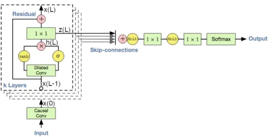
2.1. AUTOREGRESSIVE AND SEQUENCE MODELS
Figure 2.7: The dilation block that is repeated every dilation layer, is depicted inside the dotted line (these are also shown in Figure 2.9). This depicts the operations in each dilated block, and also shows the last two output layers. Adapted from [170].
boxes since in practice the computations can be done in parallel in one single convolution. However it should be understood that each yellow circle corre-sponds to it’s own separate convolution.
In the case where conditioning is applied, both convolutions get summed with another convolution which is parametrized byV where the conditioning signal isy`−1. The latter is either a scalar or a vector of the same length asx`−1
and can be obtained with the same procedure described in Figure 2.9 for the main signal: x` |{z} Ch =x`−1 |{z} Ch + Ch z }| { θ`r· h` |{z} Cres h` =τ Wf`∗x`−1+Vf`∗y`−1σ Wg`∗x`−1+Vg`∗y`−1 (2.22)
In SynthNet, the convolutions in Equation 2.22 are changed to grouped con-volutions, and in combination with the pointwise 1x1 convolution, this effec-tively results in what is called a depthwise separable convolution. This is not used in either the original WaveNet [170] nor the latter DeepVoice [9] derivative.
Skip connections Figure 2.9 depicts a standard neural network architecture where the output of each layer goes to the next and so on. However, in addition a similar idea as in DenseNets [78] is used.
There is an additional output from each dilated block in addition to x` and this is where the outputs towards the softmax come from. These are not present in the SynthNet architecture presented in Chapter 5 which uses only the top most output.
In essence, the output before the residual connection is sent towards the outputs, from each layer:
z` |{z} Ch =θ`r· h` |{z} Cres (2.23)
however before going through this convolution, only the last frame is kept, so all the z` consist of only one frame. All of these are finally stacked into one matrix and the matrix is reduced to a vector of 1 frame and Ch channels, by
summing over the layer dimension (Figure 2.9 red plus circle):
zall =relu([z1 z2 . . . zL]>) (2.24)
In other, words, all the layer outputs are collapsed onto one. Other means of performing this reduction is possible, for example by concatenating all frames (but then Ch would have to be a much smaller number) by performing a 2D
convolution over thez`stack, etc.
This is then followed by two other 1x1 convolutional layers that reduce the number of channels, up to the softmax (these are not displayed in Figure 2.9, but are visible in Figure 2.7):
zout =relu(θall·zall) (2.25)
ˆ
xt =so f tmax(θout·zout) (2.26)
Generation At generation time, autoregressive models use the output of the previous time steps in order to fill up the receptive field and generate the next output. The process is repeated until a sufficient number of frames is generated and is much slower than training. Both processes are shown in Figure 2.8.
2.1. AUTOREGRESSIVE AND SEQUENCE MODELS
Figure 2.8:Left: training an autoregressive model. Right: generation by repeated pling. In practice, padding can be added at generation time before the first actual sam-ple is generated.
Figure 2.9: Multiple dilated convolutional layers are stacked. This results in a very large receptive field, which is useful for high bandwidth data such as audio.
2.2. MULTI-TASK LEARNING
2.2
Multi-task learning
Multi-task learning, as the name suggests, refers to learning multiple (usually related) tasks in parallel or using auxiliary tasks in order to increase overall performance. MTL has many successful machine learning applications, rang-ing from speech recognition, computer vision, drug discovery to natural lan-guage processing. 2.4.2 discusses recent advances in MTL and also provides an overview of MTL methods in the context of deep learning.
I define MTL in the most general sense as possible: givenStasks{(xi,yi)Ni=11,
(xi,yi)iN=11, . . . ,(xi,yi)
NS
i=1}each with a possibly different number of observations
NS and that are either related or not, the goal is to solve problems of the form
fs : Xs → Ys, ∀s. Each task can be based on completely different data that can be of different types and can have different distributions. The core idea of MTL is to solve these multiple tasks at once, and by doing so hopefully do better overall by transferring knowledge learned on one task to improve other tasks, and vice versa (i.e. leverage task relatedness). Sometimes, additional tasks which are not of importance (i.e. auxiliary) are added in order to improve the performance of one particular task.
This chapter will demonstrate that solving multiple linear regression prob-lems of related tasks is equivalent to solving one large multi-task regression problem andvice versa.
Vector autoregression and multiclass classification VAR is a special case of MTL, as is multiclass classification. For vector autoregression and keeping the multivariate regression notation (see section 2.1, Equation 2.2 to Equation 2.5) there are problems of the form f : X→Y ⊆RS where each seriessx1,x2, . . .xs
hasNobservations,X ∈RN×Sand is parametrized byθs(and for VARθs∆). The
tasks can be related and the relationship can be described using a given matrix
A or learned from the data. More on that later on. To summarise, VAR is a special case of MTL where the input space is identical for all tasks.
Furthermore, multiclass classification is also a special case of VAR where each class is a task and all tasks have the same inputs f : X →Y ∈ {1, 2, . . . ,S}
In the next subsection I start with a generic definition of multi-task learning for linear models and the squared error. I also initially focus on the special VAR case since having the same number of examples for all tasks can lead to a cleaner notation. Then I discuss various regularization techniques and finally generalize beyond linear models to regularization for neural networks.
Solving a linear MTL problem Since Chapter 4 makes use of VAR as a special case of MTL, I start as in section 2.1 with linear models:
fs(x,θs) =θs>x (2.27)
The goal is to find the parameters θ that minimize the empirical error. This
can be done by taking the sum of the mean squared error for each task:
min θ1,...,θs S
∑
s=1 1 Ns Ns∑
i=1 (θs>xsi −ysi)2 (2.28)Then, for VAR the notation can be further simplified and written more com-pactly as exemplified in Equation 2.29. This is possible since for VAR all series are the same length and can be combined into one single matrix X (which is constructed as depicted in Figure 2.1). This implies that all tasks are fed all the series and thatyiis the output vector at examplei, for all tasks.
min θ1,...,θs 1 N S
∑
s=1 N∑
i=1 (θ>xi−ysi)2 (2.29) = min Θ 1 Nk|{z}X N×∆ Θ |{z} ∆×S − Y |{z} N×S k2F (2.30)At this point it is also a good idea to define the squared Frobenius norm, for clarity in the next paragraphs:
kAk2F =Tr(A>A) = m
∑
i=1 n∑
j=1 |ai,j|2= min{m,n}∑
i=1 σi2(A) (2.31) 322.2. MULTI-TASK LEARNING
whereσi(A)are the singular values of Aand the trace Tr is the sum of diagonal
entries of a square matrix. An interesting property of the Frobenius norm is that it is invariant under rotations.
2.2.1
Regularization for multi-task learning
A good starting point is to simply add an`2loss term for each task. This how-ever, does not produce any task dependencies:
min θ1,...,θs 1 N S
∑
s=1 N∑
i=1 (θs>xi−ysi)2+λ S∑
s=1 kθsk22 (2.32) = S∑
s=1 min θs 1 N N∑
i=1 (θs>xi−ysi)2+λkθsk22 (2.33) = min Θ 1 NkXΘ−Yk 2 F+λkΘk2F (2.34)The regularization term can be rewritten using Equation 2.31 and since the trace is invariant under cyclic permutations, and an identity matrix can be added like so:
kΘk2F =Tr(Θ>Θ) =Tr(ΘIΘ>) (2.35) This can be further rewritten as A= I:
Tr(ΘAΘ>) = ∆
∑
j=1 θ>j Aθj = S∑
s=1 S∑
k=1 ∆∑
j=1 as,kθsjθkj = S∑
s=1 S∑
k=1 as,k ∆∑
j=1 θsjθkj = S∑
s=1 S∑
k=1 as,k θs>θkIt is easy to observe now, that if A = I the diagonal elements are one when
s = k and the rest are zero. This is consistent with no task dependency since there is a weight of 1 for each task, while the weights for all other tasks are 0. Equation 2.32 corresponds to setting A = IS where each task is regularized
individually and is essentially identical to using the same input for all tasks and applying a regularizer for each task.
In order to induce task relatedness, MTL regularization amounts to weight-ing the task relatedness which can be described by a positive (semi)definite ma-trix A. The full compact notation for the general task relatedness regularization term (based on the squared loss) is:
min Θ 1 NkXΘ−Yk 2 F+λTr(ΘAΘ >) (2.36)
which also has a nice gradient:
∇L(Θ) = 2
NX
>(
XΘ−Y) +2λΘA (2.37)
showing that Equation 2.36 can be extended to other loss functions as well.
MTL regularization using graphs A special case of MTL regularization is when the graph structure of the tasks is known. For most MTL problems, there are usually groups of tasks and hence there exist multiple clusters at the
2.2. MULTI-TASK LEARNING
puts. The adjacency matrix can be used to enforce dependency between tasks via regularization by taking A = L+λI where Lis the graph Laplacian of the
adjacency matrix: A= L+λI = S
∑
s=1 S∑
k=1 as,kkθs−θkk2+λkθsk2 (2.38)howeverAis given and not inferred from the data.
Learning the task relationship matrix A If the matrix describing the relation-ships between tasks is not known, it is possible to learn it by adding an ad-ditional penalty termΩand alternating between Equation 2.41 - fitting the pa-rametersΘwhile fixingA =A∗and Equation 2.42 - finding the task relatedness
matrix AwhereΘ =Θ∗ is fixed:
min Θ,A 1 NkXΘ−Yk 2 F+λTr(ΘAΘ>) +γΩ(A) (2.39)
alternate ⇓ following eqs.
(2.40) min Θ 1 NkXΘ−Yk 2 F+λTr(ΘA∗Θ>) (2.41) min A λTr(Θ∗ AΘ > ∗) +γΩ(A) (2.42)
One possible choice forΩis Tr(A−2). Looking at the Frobenius norm (Equa-tion 2.31) and the output space rota(Equa-tion trick in paragraph 2.2.1 this amounts to
γ∑s(1/σs2). This ensures that task importance will not vanish for any task.
MTL regularization computations Assuming that the matrixAin Equation 2.36 is symmetric positive (semi)definite, then it is possible to diagonalize the matrix via singular value decomposition (SVD)A =UΣU>whereΣ =diag(σ1,σ2, . . .σs).
Then, setting ˜Θ =ΘUand ˜Y =YU it is possible to rewrite Equation 2.36 as: min Θ 1 NkXΘ˜ −Y˜k 2 F+λTr(ΘΣ˜ Θ˜>) (2.43)