Consumer Credit Scoring

C

ONSUMER

C

REDIT

S

CORING

Alexandru CONSTANGIOARA1

A

bstract

After presenting the main issues in consumer credit market and introducing the issue of credit scorecards, I have used statistical modeling to predict the default probabilities of applicants in a dataset of consumer loans. I have found evidence for the superior accuracy of complex non-linear estimations. In particular, the bagging model offers better results than the traditional tree and logit estimations. The proposed statistical scorecard offers a 60 percent improvement over the baseline model. Lastly, this paper argues that the management must establish a decisional probability threshold in accordance with its propensity for risk. A higher threshold requires a greater promotional effort, although the increased costs may be compensated by a more efficient communication with clients and by more flexible contractual clauses.

Keywords: credit market, prudential regulation, statistical scorecards, logit, bagging estimations

JEL Classification: C13, G21

I

. Introduction

After the 1980’s, the consumer credit market has shown a significant increase, both in the value of outstanding amount and in the value of consumer credit relative to GDP and households revenues (Siddiqui, 2006). Empirical studies show that the development of market has led to over-indebtedness and consumer bankruptcy phenomena. Increasing competition has fueled aggressive marketing techniques, which resulted in a deeper penetration of the customers’ pool, and, especially, of low income customers that usually carry a higher debt burden, pay more interest and suffer more defaults (Niu, 2004). Under these circumstances, the risk management of consumer lending has become critical to protect the interest of both lenders and consumers (Siddiqui, 2006).

There are two major categories of risk in the market: systemic risk and credit risk. Effective regulations and laws provide a safeguard for the industry from shocks that might pose a systemic risk. Since the early work of Durant (1941), there has been considerable interest in using statistical tools and risk management strategies to cope

1 _{Oradea University, Faculty of Economic Studies, E-mail: [email protected],}

[email protected]

with credit risk. Hand and Henley (1997) offer a summary of the statistical methods used in the industry to predict credit risk.

The current paper, after presenting the main evolutions in the consumer credit in the EU and a brief overview of the Romanian consumer credit market, focuses on the development of a statistical scorecard for the selection of credit applications. I have evaluated the comparative efficiency of several statistical methods available in consumer credit scoring and I have developed a statistical scorecard. This paper documents the superiority of complex non-linear estimations. In particular, the bagging model offers better results than the traditional tree and logit estimations. Following the existing empirical studies on credit risk, I used the weight of evidence variables (WOE) as inputs in estimating the predicted default probabilities. Using WOE preserves the distribution of good and bad accounts in the population and avoids an arbitrary ordering of categorical variables, which ultimately translates into more reliable credit scorecards.

II

. The Consumer Credit Market

The consumer credit products cover general-purpose loans (personal loans), revolving credit (with or without a plastic card), loans linked to specific purchase (such as point-of-sale finance for cars and consumer durable goods), but not residential mortgage business (Guardia, 2000). In general, the consumer credit is not guaranteed whereas mortgage credit uses property as collateral. The distinction between consumer and mortgage credit is also underlined in the Consumer Credit Directive, adopted by the European Commission in May 2008, with June 2010 as date for completing the transposition for all the member states.

The consumer credit is difficult to measure for several reasons. In the developing countries, the consumers arbitrage between consumer and mortgage credit, using the cheaper mortgage credit for other purchases than property (Guardia, 2000). This phenomenon has blurred the distinction between consumer and mortgage credit. Another shortcoming is that most countries report the consumer credit outstanding (stock measure), which is different from the consumer credit flow (Guardia, 2000).

2.1 Evolution

There are three main activities within consumer credit financing: vehicle financing, point-of-sale financing, and direct financing. Vehicle financing is one important activity within consumer credit, ranging between one fifth and two thirds of the consumer credit outstanding. Vehicle financing is less important in the UK and France (15 percent of the total outstanding), whereas at the other end of the spectrum we find Spain, Germany and Italy, with 35, 40 and 60 percent of the total outstanding (Mercer Oliver Wyaman, 2005). Today, most European countries have vehicle financing markets that involve banks and specialists, often for both new and used cars. In most countries, the dealer channel represents the main source for financing. Point-of-sale (POS) financing, the second important segment of consumer credit market, offers credit facilities. It covers durable goods and services, such as travel, health and entertainment. Similar to vehicle financing, POS financing offers the customers a

credit facility. This segment covers on average 10 percent of total outstanding, varying from only 5 per cent in Germany to 33 per cent in France and 22 per cent in Spain (Mercer Oliver Wyaman, 2005). The concentrated retail markets in France and Spain made POS financing a key element of consumer credit market. Direct financing, a relatively new form of financing, has outpaced vehicle and POS financing. This segment is more developed in Germany and the Netherlands and less developed in Italy, France and Spain. The direct financing segment has two main characteristics: the customer establishes a direct relationship with the financing entity and the loan is not linked to a specific purchase.

Consumer credit outstanding in the EU-27 amounted to around €884 bl. at the end of 2008, representing 7 percent of the EU GDP. If we consider the non-banking financial institutions, the consumer credit market amounts to approximately €1236 bl., or 10 percent of the member states’ GDP. In Europe, where data show strong concentration, the three largest consumer credit markets are the United Kingdom, Germany and France. The six largest EU economies amount to 80 percent of the European credit market (GHK Consulting, 2009).

In the EU, the growth pattern has been uneven across member states. Until recently, the consumer credit markets exhibited strong growth in the new member states. This was due to several factors, including the relative buoyancy of household consumption, increasing competition among credit institutions in the market and diversification of the range of financial product offering and new distribution channels, such as Internet and mobile phone technology. In the historically constrained consumer credit markets of the new entrants, banking liberalization and foreign investments have also fueled a surge in borrowing. Within the EU-12, consumer borrowing is the highest relative to GDP in Cyprus, with 25.1 percent and Poland, with 22.7 percent (GHK Consulting, 2009).

A major concern regarding the consumer credit market is the increasing over-indebtedness. For debtors, the extent of the impact of over-indebtedness on households’ capacity to service their debt is the most relevant. Rinaldi and Sanchis (2006) document the households’ capacity to service debt in spite of the development of new financial products and of deeper penetration of the market. However, Bridges and Disney (2003), using the Survey of Low Income Families in the UK, found evidence of increasing debt and arrears among the low income families.

To address the over-indebtedness phenomenon, regulation is essential. Regulation ensures a fair, safe and competitive market environment serving all the stakeholders. In several central and northern European countries, the judicial debt adjustment laws are already in place and the EU legislation already addressed the problem of cooperation in this field. However, according to the Consumer Credit Directive (2008), aspects such as consumer protection, debt collection and debt enforcement still have to be addressed in order to promote an open and fair consumer credit market, where consumers can make fully informed decisions and businesses can compete aggressively on a fair and even basis.

The 2008 financial crisis severely curtailed the lending capacity of the financial institutions. This has hindered the fast development of lending to households within the EU. Consequently, the outstanding stock of consumer credit has fallen in most EU

countries. On the consumers’ side, the crisis negatively affected their capacity to service debt. Both the previous empirically documented increased indebtedness (Niu, 2004) and the financial crisis contributed to the worsening of households’ capacity to service debt, making the risk management of consumer lending critical to protect the interest of both lenders and consumers.

2.2 Overview of the Romanian Consumer Credit Market

The Romanian consumer credit market exhibited strong growth until recently. In Romania, the consumer credit outstanding represented 13.7 percent of GDP at the end of 2008 (as compared to 9.9 percent in the EU-27 and 8.8 per cent in the Euro Zone). While a country’s consumer credit outstanding can be used to evaluate its market size and growth, the consumer credit per capita is more suited for comparing different countries on an equal basis. The average consumer credit outstanding per capita in Romania in 2008 amounted to € 873, which represented only 31 percent of the EU-15 average (GHK Consulting, 2009). This is unsurprising, reflecting the remaining development gap between Romania and the EU-15.

Starting with 2008, the demand for loans was negatively affected by the slowing down business activity, increasing trend in inflation and deteriorating exchange rate. Prudential regulation enacted by NBR also curtailed the credit supply, in order to prevent further deterioration of credit portfolios. In 2009, the consumer credit dynamics slowed down to -3.6 in real terms as compared to the previous year. Moreover, the uncertainties of the global financial crisis induced the worsening of banks’ loan portfolios. Thus, the share of non-performing loans (loans overdue for more than 90 days and/or for which legal proceedings were opened) increased from 2.8 percent at the end of 2008 to 7.9 percent at end of 2009 and to 10.2 in June 2010 (2010 NBR Report).

Starting in the second quarter of 2010, the measures taken by NBR to support the priority economic sectors and to facilitate the individuals’ access to house purchasing have finally stopped the decreasing trend in non-governmental loans, which would ultimately impact positively on the evolution of the consumer credit (2010 NBR Report).

It must be underlined that by stimulating loans for the economy the NBR responded to the strong criticism of the pro-cyclicality induced by Basel II capital requirements (Caprio, Levine, 2002). In fact, the new regulatory framework on capital proposals (Basel III) acknowledges the need to address the pro-cyclicality issue through dynamic provisioning based on expected losses (Blundell-Wignall, Atkinson, 2010). The current financial crisis revealed major deficiencies in the operation and regulation of the financial system, providing an impetus to the efforts of restructuring and consolidating its architecture. The crisis also revealed deficiencies in the existing deposit-guarantee schemes at EU level. Consequently, the EU legislators decided that it was a priority to restore confidence and proper functioning of the financial sector by protecting de deposits of individual savers, bringing forward a proposal to promote the convergence of the deposit-guarantee schemes (Directive 2009/14/EC).

The prudential measures enacted by the NBR are not enough to protect the interest of consumers in the consumer credit market. A key objective of the new Consumer

Credit Directive is to provide a high level of protection for all the consumers in the Community. An extensive study of the consumer credit in the EU has documented prima facie evidence of imperfections in the market that may affect the retail financial services, in general, and the consumer credit markets, in particular (GHK Consulting, 2009). In particular, inadequate information may make consumers select the wrong product for their needs or to select a product of poor value as compared to other available products. While all the EU countries are facing inadequate information on the part of the consumer, the situation is particularly worrisome in Romania, where the European Database for Financial Education identifies only one financial literacy scheme, as compared to 11 in Poland, 43 in Denmark or 78 in the UK (GHK Consulting, 2009).

III

. Credit Scorecards

While prudential regulation and regulation aimed at removing the existing barriers in the consumer credit market are prerequisites for the development of the Romanian consumer credit market, the current paper focuses on the usage of statistical tools to evaluate better the credit risk in the market.

3.1 Scorecards: General Overview

Credit scorecards are the main tool used in assessing the credit risk in the consumer credit market. Credit scores indicate the trade-off between the risks and the penetration of the market, measured by depth, breadth and length. The depth shows the targeted segments, the breadth shows the penetration of each segment and the length measures the profits obtained. Since the risk is better evaluated, the scoring will increase the companies’ efficiency. Risk scoring, in addition to being a tool to evaluate the risk associated with applicants or customers, proved to be efficient in other operational areas, too. For example, the risk scoring assists the decision-making process. Borderline applications are given to more experienced staff for additional scrutiny, while low risk applications are assigned to junior staff. In addition, credit scoring improves the quality of portfolios intended for acquisition (Siddiqui, 2006). There are three types of credit scorecards. Subjective scoring is based mainly on intuition. However, Schreiner (2003) shows that it uses qualitative judgment and even quantitative guidelines to evaluate the creditworthiness of applicants. The main advantage of subjective scoring is convenience; in its case, there is no need to build a credit history database. Of course, this comes at the expense of inadequate predictive accuracy and subjective judgment. Expert systems provide the second category of scorecards. They are derived from the experience of managers and loan officers. While subjective scorecards use mainly implicit judgment, expert systems are based on explicit rules, statistics or mathematics. The simplest expert system is a decisional tree whose splits come from experience and not from statistical analysis of the data. However, statistical analysis can be used to control the growth of the tree. The third type of scoring uses statistical analysis to predict the credit risk explicitly as a probability. While statistical scorecards do not identify good or bad applications on an individual basis, they provide statistical odds or the probability that an applicant will

default. Default probabilities and business considerations (expected profit, losses) are then used for decision-making. In its simplest form, a statistical scorecard consists in a group of characteristics, statistically determined to be predictive in separating the two classes of applicants (bad and good). The total score of an applicant is the sum of the scores for each attribute present in the scorecard for that applicant.

3.2 Statistical Methods Used in Credit Scoring

A summary of the statistical methods for assessing credit risk is offered by Hand and Henley (1997). Statistical scoring uses predictor variables to yield probabilities of default or to predict the repayment behavior of borrowers. Schreiner (2003) argues that regression estimations, discriminant analysis and decisional trees are the most prevalent statistical methods used in assessing the credit risk. However, more sophisticated methods, such as nonparametric smoothening, mathematical programming, Markov chains, recursive partitioning, genetic algorithms or neural networks are also available.

Binary logit and probit models

Probit and logistic regressions derive the probability of the event of interest based on the equation:

)

1

(

)

(

1

)

0

(

)

1

(

prob

b

X

U

F

b

X

Y

prob

!

The logit model assumes a logistic distribution of the error term, while the probit model assumes standard normal distribution of Ui.Therefore, the probability of interest is:

For logit model:

(

2

)

)

exp(

1

)

exp(

)

|

1

Pr(

bX

bX

X

Y

For probit model:

)

(

3

)

2

exp(

)

2

(

)

|

1

Pr(

dz

z

X

Y

³

S

The parameters are estimated by maximum likelihood, which maximizes a probit likelihood function for the probit model and a logit likelihood function for the logit model.

Logit and probit estimation of credit risk received a lot of attention in the credit risk literature. On theoretical grounds, they are considered a more appropriate statistical tool for estimating probabilities than the linear probability model. As Schreiner (2003) shows, empirical results tend to agree with theoretical predictions. Nevertheless, Hand and Henley (1997) argue that if a large proportion of the applicants have estimated default probabilities between 0.2 and 0.8, the logistic and normal curve are well approximated by a straight line and the Linear Probability Model can provide similar results.

Neural Networks

In data analysis, artificial neural networks are a class of flexible nonlinear models used for supervised prediction problems. Because of the analogy to neurophysiology, they

are usually perceived to be more glamorous than other prediction models. Multi-layer perceptron models were originally inspired by neurophysiology and the interconnections between neurons. The structure of a multi-layer perceptron is represented by a network diagram. Each element in the diagram has a counterpart in the network equation. The model parameters are given random initial values, and predictions of the target are computed. These predictions are compared to the actual values of the target, via an objective function which minimizes the difference between the actual and predicted values of the target. Training proceeds by updating the parameter estimates in a manner that decreases the value of the objective function. Training concludes when small changes in the parameter values no longer decrease the value of the objective function. The network is said to have reached a local minimum in the objective. At convergence, the model is likely to be highly generalized. The overall average profit is examined to compensate for over-generalization. The final parameter estimates for the model are taken from the iteration with the maximum validation profit (George, 2001). One should note that the coefficients of a nonlinear model are not directly interpretable (Wooldridge, 1999), not to mention that in the case of a neural network to interpret them is futile.

Decisional tree

Recursive partitioning models, commonly called decision trees are the most prevalent predictive modeling tool, although they may not yield the largest generalization profit. They do not assume a particular functional relationship, which allows them to find complex relationships between target and inputs. It also allows them, if not carefully tuned, to over-generalize. The tree algorithm is very complex. The first part of the algorithm identifies the best split for each variable, by using, for example, a Pearson chi-squared statistic to quantify the independence of counts resulted. Large values for the chi-squared statistics suggest that the proportion of 0’s and 1’s in the left branch is different than the proportion in the right branch. The resulting partition of the input space is known as the maximal tree. Development of the maximal tree was based exclusively on statistical measures of split worth on the training data. It is likely that the maximal tree will fail to generalize well on an independent set of validation data. The second part of the tree algorithm, called pruning, attempts to improve generalization by determining the optimal tree, based on profit maximization (Potts, 2001).

Tree analysis is often used for the initial data analysis, mainly for exploratory purposes. Sometimes, the analysts use tree analysis as an auxiliary tool for building more complex models, such as logistic regressions. The reason for this is because tree algorithm can deal directly with missing values, whereas regressions, for example, do not have this ability.

Bootstrapping aggregation (bagging)

Decision trees are unstable models. Small changes in the training data can cause large changes in the topology of the tree, yet leaving the results unaltered. The overall performance of the tree remains stable (Breiman, 1996). The instability comes from

the large number of univariate splits considered. At each split, there are typically a number of splits on the same inputs that give similar performance. Methods have been devised to take advantage of the instability of the trees. The Perturb and Combine (P&C) methods generate multiple models by manipulating the distribution of the data or altering the construction method and then averaging the results. Any unstable method can be used, but trees are most chosen because of their speed and flexibility.

The attractiveness of P&C methods is their increased performance over single methods (Bauer and Kohavi, 1999). One reason for this is simply variance reduction. If the base model has low bias and high variance, then averaging reduces variance. In contrast, combining stable models can negatively affect performance.

Bagging (bootstrap aggregation) is the original P&C method. First, a number of bootstrap samples are selected randomly. Then, a tree is constructed on each sample. Finally, the ensemble model is constructed by voting on the classification or averaging the posterior probabilities.

IV

. Credit Risk Analysis Using a Dataset of

Consumer Loans

The current analysis uses econometric modeling to estimate the default probabilities associated with a consumer credit loan. There are several issues that might bias the analysis of credit risk. A first issue is that the monitoring period of arrears is short, which raises the question regarding the maturity of the accounts. Immature accounts are considered those which do not have time to “go bad”. In practice, behavioral scorecards need to rely on at least a two-year observation period (Siddiqui, 2006). On the other hand, using data on existing accounts to predict default probabilities is problematic because of selection bias issue - the default accounts are not selected randomly from the sample of applicants. Siddiqui (2006) stresses that the developing sample must include an equal number of defaults, non-default and rejected cases. An adequate solution for this problem would be to estimate a system of equations, one for default probability and the other for the probability that one receives a loan. Another issue that might compromise the results is the population drift. This refers to changes over time in the distribution of population. This issue is particularly relevant for transition economies, as Natasa Sarlija et al. (2007) found in a study using Croatian data.

4.1 Data and Variables

I have used a Hungarian dataset of 5060 observations of existing accounts of loans for personal needs. Data comes from the Budapest Banking Institute. Analysis uses three groups of variables. A first group consists of demographic characteristics. A second group of variable refers to the financial situation of the borrower and the third refers to the loan and re-payment history. The old scoring date variable has been used to determine the tenure of the accounts. The examination of variables, corroborated with the test of equality of group means show that default accounts have higher net income than the non-default cases. The other variables offer no surprises:

default cases are associates with less educated, single, younger persons, with less tenure with current employer.

4.2 Default Probabilities and the Efficiency of the Models

As recommended by existing data mining soft packages, I have used a 70:30 partition of the dataset. Several soft packages were used (in most cases, SPSS and EViews). Missing observations were replaced using a standard procedure offered by the employed software. The procedure is needed because missing observation can negatively affect parametric estimations that suffer from over-dimensionality. Observations have been interactively grouped by computing the weights of evidence (WOE) variables. WOE variables are defined as the log ratio of the distribution of good accounts to the distributions of bad accounts. Using WOE preserves the distribution of good and bad accounts in the population and avoids an arbitrary ordering of categorical variables, which ultimately translates into more reliable credit scorecards (Siddiqui, 2006). To model the default probabilities, I have used logit, neural, tree and bagging estimations.

Logit estimation of default probabilities

As mentioned, logit estimation uses WOE as input variables. I have employed a stepwise selection of the variables, ensuring a high statistical significance of the model and the estimates (P<0.05). The main results are presented in Table 1.

Table 1 The Main Results of Logit Estimation

Variable (label) Coefficient p-value Variable (label) Coefficient p-value

Intercept -4.65 0.01 Income -0.96 0.00

Age -1.21 0.00 Old score -0.57 0.03

Education -0.97 0.00 Tenure -0.75 0.01

Employment sector 0.71 0.04 Family members -0.83 0.00 Family income -0.78 0.00 Marital status 0.26 0.00 Free income -0.65 0.00

Variables that were found to be significant are broadly the same as those reported in previous empirical literature. Natasa Sarlija et al. (2007) argues that for consumer credit scoring the variables found to be significant in empirical studies are time at present address, marital status, postcode, telephone, applicant's annual income, owing a credit card, type of bank account, age, type of occupation, purpose of loan, time with bank, time with employer, credit office rating, monthly debt as a proportion of monthly income, time at current job and number of dependents. As Table 1 shows, the coefficients corresponding to income variables are negative.

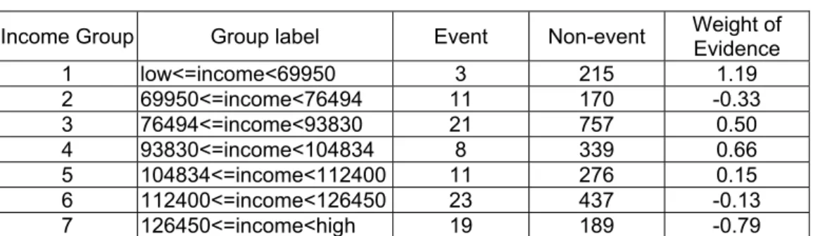
The reason for the negative sign of the coefficients corresponding to the income variable is the sign of WOE values, reported in Table 2. As shown in Table 2, a high income corresponds to a negative WOE value, whereas a low income corresponds to a positive WOE value.

Table 2 The WOE Values for the Income Variable

Income Group Group label Event Non-event Weight of Evidence 1 low<=income<69950 3 215 1.19 2 69950<=income<76494 11 170 -0.33 3 76494<=income<93830 21 757 0.50 4 93830<=income<104834 8 339 0.66 5 104834<=income<112400 11 276 0.15 6 112400<=income<126450 23 437 -0.13 7 126450<=income<high 19 189 -0.79

Consequently, moving from a high to a low income reduces the default risk. Although this is somehow counterintuitive, it corresponds to previous findings in empirical credit risk literature. Mark Schreiner (2003) considers that the positive partial effect of income on default probability might be attributable to other personal characteristics associated with higher income. Table 1, according to the same line of reasoning shows that default risk is negatively associated with the number of children. Moreover, we see that unmarried persons have a higher associated default probability than married ones. In other words, marriage and kids act as a proxy for personal characteristics associated with non-delinquent credit behavior. Table 1 also shows that education and age have the expected effect on default risk: higher values for education and age reduce the default risk. The employment sector also affects significantly the credit risk. Working for the private sector increases the estimated default risk, probably due to the higher volatility of employment which characterizes this sector. As expected, Table 1 shows that tenure and the old score are negatively associated with default risk. The overall accuracy of logit estimation is 4 percent, both for estimation and validation set.

Neural estimation of default probabilities

The optimization function converges after 8 iterations. The average misclassification rate for neural estimation is 4 percent for both validation and estimation set. The final prediction error of the model is 4 percent. Although the complexity of neural networks allows them to approximate virtually any continuous association between the inputs and the target by simply specifying the correct number of derived inputs, it is virtually impossible to interpret the coefficients of the neural network estimations. Consequently, neural networks cannot be used for the development of traditional credit scorecards, based on clearly defined adjudication rules.

Tree estimation of default probabilities

I have used SPSS for estimating a tree model of default probabilities. Once again, I have used a 70:30 partition of the initial dataset. The main results for the estimation set are presented in Table 3.

Table 3 The Main Results of Tree Modeling

STAT ARREARS 0 1 TOTAL

N 0 3385 0 3385

N 1 156 0 156

Col% 0 96 0 96

Col% 1 4 0 4

One may see that tree modeling is unable to discriminate between good and bad accounts. While all of the non-defaulting cases are correctly identified, tree modeling fails to identify the default cases. However, the overall prediction accuracy of the model is the same as that of previous models (96 per cent). The prediction accuracy stays the same regardless of tree depth.

Bagging estimation of default probabilities

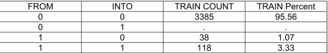
The current analysis uses 100 iterations for the bootstrap sampling. Decision tree modeling has been employed to obtain default probabilities for each sample in part. In the final stage, the ensemble model has been obtained by averaging across results. As mentioned before, bagging, one of the most used P&C methods, uses the instability of individual tree modeling in order to reduce the variance of the estimations. The main results of the bagging estimation for the estimation set are presented in Table 4.

Table 4 The Classification Table for the Bagging Estimation of Default

Probabilities

FROM INTO TRAIN COUNT TRAIN Percent

0 0 3385 95.56

0 1 . .

1 0 38 1.07

1 1 118 3.33

Table 4 shows that misclassification rate drops to 1 percent, as compared to 4 percent for the other models. Most importantly, we see that bagging is efficient in discriminating between the two classes of accounts: in the estimation set the model correctly identifies 118 out of the 156 bad accounts, which is unquestionably a good performance. However, the accuracy of bagging modeling for the validation set is 4 percent, as for the other models employed in the analysis.

4.3 The Efficiency of the Models

The efficiency of a predictive model is optimally measured by the overall average profit on a set of validation data. Accuracy, the most obvious measure of a model’s worth, is a special case of the general profit structure. Correct decisions are rewarded with a one unit profit. Incorrect decisions receive zero profit. The expected profit for a decision simply equals the probability of the corresponding target level. Thus, the best

decision for each case corresponds to the most likely target value. The overall average profit is the total number of correctly decided cases divided by the total number of cases. Maximizing the overall average profit by this simple profit structure is identical to maximizing accuracy.

Based on accuracy, all the models in the analysis have the same results for the validation set: a misclassification rate of 4 percent. The models do very well in predicting non-default cases. Predicting default cases depends on the target threshold. For a 50 percent threshold none of them is able to identify correctly the bad accounts. However, this is not surprising considering the sample proportion of the default cases (~4 percent).

The ROC curve, a visual index of the accuracy of the models, provides additional information on the efficiency of the estimations. Once again, the analysis shows similar results. The area below the ROC curve is 0.748 for logit, neural and bagging and 0.742 for tree estimation. All the corresponding p values are 0.00, which reveals a high statistical significance of the results. Based on the ROC analysis, I conclude that tree estimation is less accurate than the other estimations employed in this paper. Consequently, the subsequent analysis will concentrate on the comparative accuracy of logit, neural and bagging models.

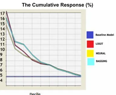
The subsequent analysis is based on the response and captured response charts. These tools are widely employed in credit scoring. The response chart arranges observations into deciles. Observations are sorted in descending order of their predicted probabilities of default and the plotted values are the actual probabilities of default. The non-cumulative plot shows the percentage of defaulters in each decile. The cumulative graph (Figure 1) averages the non-cumulative percent response across deciles (therefore, for 100 percent of the estimated predicted probabilities the average equals the value for the baseline model).

Figure 1 The Cumulative Response (%)

If the model is useful, the proportion of actual defaults will be higher in top deciles and the plotted curve will be descending in both cases (cumulative and non-cumulative cases).

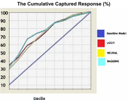
Figure 1 shows that for the logit estimation the actual proportion of default cases for the first decile is 18 percent, as compared to 16 percent for bagging. For the next three deciles, Figure 1 shows an actual proportion of cumulated default cases of 11.5, 11 and 9 percent for bagging, whereas the corresponding figures for logit are 11, 9 and 8 percent. We can conclude based on these results that, although for the first decile logit estimation offers better results, bagging estimation clearly outperforms logit and neural estimations. Figure 1 also shows that all cumulative response charts are descending, which clearly underlines that they are useful in differentiating the two classes of accounts. The cumulative captured response curve (Figure 2) shows what percentage of the total defaulters are in a bin. The proportion of defaulters in the first decile is approximately the same for logit and bagging (32 percent), whereas bagging offers better results for deciles two, three, and four.

Figure 2 The Cumulative Captured Response (%)

Based on cumulative response and cumulative captured response charts, we can conclude that bagging outperforms logit and neural estimations in terms of accuracy.

4.4 The Development of a Statistical Scorecard for Selecting the Consumer Credit Applications

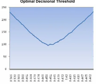
Since previous analysis has documented the superior accuracy of the bagging estimation, I use bagging estimated default probabilities for the construction of the credit scorecard. More detailed analysis of the two charts (cumulative response and cumulative captured response charts) shows that the optimal decisional threshold is

0.451. For this probability, the number of wrong decisions (false positive plus false negative) is minimized (Figure 3).

Figure 3 Optimal Decisional Threshold

As depicted in Figure 3, a 0.451 decisional threshold results in 95 wrong decisions compared to the corresponding 231 bad accounts in the original sample. Thus, the proposed statistical scorecard offers a 60 percent improvement over the baseline model. One should note, however, that the management must establish a decisional probability threshold in accordance with its propensity for risk. A greater propensity for risk on its part increases the threshold above the 0.451 value, but such an option has its costs. Obviously, a higher threshold requires a greater promotional effort, due to increased attention allocated to critical accounts. The increase in costs might be compensated by a more efficient communication with clients and by more flexible credit contracts.

V

. Concluding Remarks

Increasing competition in the consumer credit market has fueled aggressive marketing techniques, which have resulted in a deeper penetration of the customers’ pool, and especially of low income, riskier customers. The risk management of consumer lending has become critical to protect the interest of both lenders and consumers. The paper analyzes the issue of consumer credit scoring. After presenting the main issues in consumer credit market and introducing the credit scorecards, I used

statistical modeling to predict the default probabilities of applicants in the dataset. I have shown the superiority of WOE as inputs in credit risk modeling. I have found evidence for the superior accuracy of complex models such as bagging, logit and neural over traditional tree estimation. Using tools specific to credit risk industry, I documented the superior accuracy of bagging model over logit and neural model. I used bagging estimated default probabilities for the construction of a credit scorecard. Detailed analysis of the cumulative response and cumulative captured response charts shows that the optimal decisional threshold is 0.451. The proposed statistical scorecard offers a 60 percent improvement over the baseline model. Lastly, I have underlined that the management must establish a decisional probability threshold in accordance with its propensity for risk. A greater propensity for risk on its part increases the threshold above the 0.451 value, but such an option requires a greater promotional effort and a more efficient communication with clients.

R

eferences

Bauer, E. and Kohavi, R., 1999. An Empirical Comparison of Voting Classification Algorithms: Bagging, Boosting and Variants. Machine Learning, 36(1-2), pp.105-139.

Blundell-Wignall, A. and Atkinson, P., 2010. Thinking Beyond Basel III. Necessary Solutions for Capital and Liquidity. Financial Market Trend, 1.

Breiman, L., 1996. Bagging Prediction. Machine Learning, 24, pp.123-140.

Bridges S. and Disney R., 2001. Modeling Consumer Credit and Default: The

Research Agenda. Experian Centre for Economic Modeling (ExCEM):

University of Nottingham Press.

Caprio, G., Levine, R., 2002. Financial Regulation and Performance: Cross Country Evidence.Central Bank of Chile, Working Paper no. 118.

Diez G., 2000. Consumer Credit in the European Union. ECRI Press.

Directive of the European Parliament and the Council on Credit Agreements for Consumers and Repealing Council Directive 87/102/EEC., 2008. Available at: <http://www.eccromania.ro/legislatie/creditul-de-consum/directive-48-2008-consumer-credit-en/view> [Accessed on December 2009].

Durand, D., 1941. Risk Elements in Consumer Instalment Financing. NY: National Bureau of Economic Research.

George, J., 2001. Predictive Modeling Using Enterprise Miner. SAS Institute Inc., Chapter 2.

Georgescu, G., 2005. Stadiul Pregatirii Pentru Aplicarea Reglementarilor BASEL II in

Sistemul Bancar Romanesc. BNR.

GHK Consulting, 2009. Establishment of a Benchmark on the Economic Impact of the Consumer Credit Directive on the Functioning of the Internal Market in

This Sector and on the Level of Consumer Protection. DG Health and

Hand D. and Henley W., 1997. Statistical Classification Methods in Consumer Credit Scoring: A Review. Journal of the Royal Statistical Society, 160(3), pp.523-541.

Mercer Oliver Wyaman, 2005. Consumer Credit in Europe: Riding the Wave. ECRI Press.

National Bank of Romania, 2008. Annual Report. Available at: <http://www.bnro.ro/PublicationDocuments.aspx?icid=6877>

[Accessed on December 2009].

Niu, J., 2004. Managing Risks in Consumer Credit Industry. In: China Center for Economic Research, Policy Conference on Chinese Consumer Credit. Beijing, China, August 7, 2004.

Potts, W., 2001. Decision Tree Modeling. SAS Institute Inc., Chapter 1.

Rinaldi, L. and Sanchis-Arellano A., 2006. Household Debt Sustainability. What Explains Household Non-Performing Loans? An Empirical Analysis.

European Central Bank, Working Paper Series, No. 570.

Sarlija, N. Bensic, M. and Bohacek, Z., 2007. Customer Revolving Credit – How the Economic Conditions Make a Difference. In: The University of Edinburgh Management School, Credit Scoring & Credit Control 10th

Conference.

Schreiner, M., 2003. Scoring: The Next Breakthrough in Micro Credit? Occasional Paper No 7.

Siddiqui, N., 2006. Credit Scorecards. John Wiley&Sons Inc., Ch. 1, 2, 3 and 7.

Wooldridge, J., 1999. Introductory Econometrics. South Western College Publishing, Ch. 17.