Genetic Process Mining:
An Experimental Evaluation
A.K. Alves de Medeiros
∗
, A.J.M.M. Weijters
and W.M.P. van der Aalst
Department of Technology Management, Eindhoven University of Technology P.O. Box 513, NL-5600 MB, Eindhoven, The Netherlands.
Abstract
One of the aims of process mining is to retrieve a process model from an event
log. The discovered models can be used asobjective starting points during the
de-ployment of process-aware information systems (PAIS) [19] and/or as a feedback mechanism to check prescribed models against enacted ones. However, current tech-niques have problems when mining processes that contain non-trivial constructs and/or when dealing with the presence of noise in the logs. Most of the problems
happen because many current techniques are based onlocalinformation in the event
log. To overcome these problems, we try to use genetic algorithms to mine process
models. The main motivation is to benefit from theglobal search performed by this
kind of algorithms. The non-trivial constructs are tackled by choosing an internal representation that supports them. The problem of noise is naturally tackled by the genetic algorithm because, per definition, these algorithms are robust to noise. The main challenge in a genetic approach is the definition of a good fitness measure because it guides the global search performed by the genetic algorithm. This paper explains how the genetic algorithm works. Experiments with synthetic and real-life logs show that the fitness measure indeed leads to the mining of process models
that are complete (can reproduce all the behavior in the log) and precise (do not
allow for extra behavior that cannot be derived from the event log). The genetic algorithm is implemented as a plug-in in the ProM framework.
Key words: process mining, genetic mining, genetic algorithms, Petri nets, workflow nets.
∗ Corresponding author.
1 Introduction
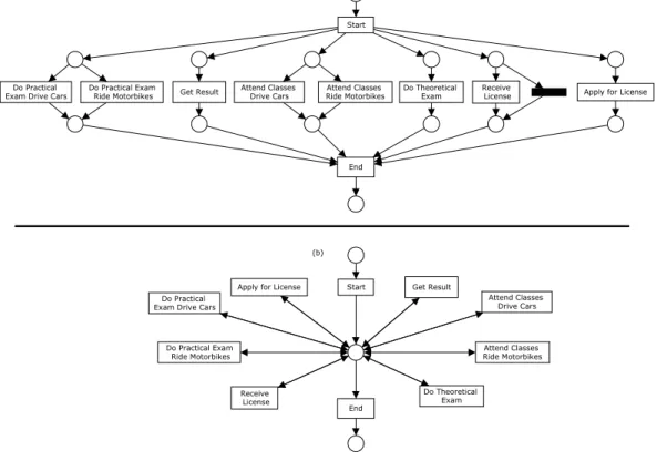
Today’s organizations are supported by a wide variety of information sys-tems. Some systems only support a single task (e.g., a text editor). However, most organizations are using systems that support processes, i.e., not a sin-gle task but the glue between tasks. Examples are WorkFlow Management (WFM) systems and Enterprise Resource Planning (ERP) systems. Typically, these systems record events that can be linked to the execution of some task in the process. Therefore, it makes sense to analyze these events to get feed-back about enacted processes. Buzzwords such as Business Process Intelligence (BPI) and Business Activity Monitoring (BAM) indicate the interest of orga-nizations and software developers in solutions able to extract knowledge from so-called event logs. However, most of the commercial systems (e.g., Cognos and Business Objects) focus on exclusively performance issues such as flow time and utilization. These systems abstract from the process itself and can only be applied if the process is well-defined and fixed. ARIS PPM is one of the few commercial systems actually trying to discover more information by monitoring events. One of the reasons for this limited support is that it is very difficult to extract process knowledge without having some a-priori pro-cess model. This triggered the development of propro-cess mining techniques that aim at automatically discovering process models based on event logs.
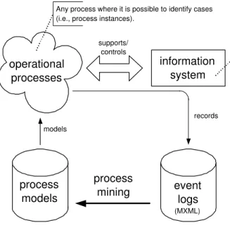
information system operational
processes
process
models eventlogs
(MXML) models process mining records supports/ controls
Any system supporting operational processes while recording events in, e.g., some transaction log or audit trail. Examples include workflow management systems (e.g., Staffware), enterprise resource planning systems (e.g., SAP R/3), product data management systems (e.g., Windchill), hospital information systems (e.g., Siemens Soarian), case handling systems (e.g., FLOWer), customer relationship management systems (e.g., Microsoft CRM), webservice composition systems (e.g., Oracle BPEL), etc. Any process where it is possible to identify cases
(i.e., process instances).
Fig. 1. Overview of process mining.
Figure 1 illustrates the concept of process mining. Some operational process is supported by some information system that records events in some event log. This event log is used to extract process models that describe the observed behavior. This information is valuable to better understand processes and to improve them. In our experience, real processes tend to deviate from the
idealistic processes people have in mind. The practical relevance of process
mining is obvious. Unfortunately, existing techniques have severe limitations1.
Therefore, we present a new approach using a genetic algorithm. However, before we introduce our approach, we first need to clarify the concept of process mining.
1.1 Process Mining
One of the aims of process mining is to automatically build a process model
that describes the behavior contained in an event log. The models mined
by process mining tools can be used as an objective starting point during
the deployment of systems that support the execution of processes and/or
as a feedback mechanism to check the prescribed process model against the
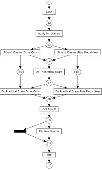
enacted one. We use an example to illustrate how process mining techniques work. Consider the event log shown in Table 1. This log shows the event traces (process instances) for four different applications to get a license to ride motorbikes or drive cars. Note that applicants for different types of licenses do the same theoretical exam (task “Do Theoretical Exam”) but different practical ones (tasks “Do Practical Exam Drive Cars” or “Do Practical Exam Ride Motobikes”). In other words, whenever the task “Attend classes Drive Cars” is executed, the task “Do practical Exam Drive Cars” is the only one that can be executed after the applicant has done the theoretical exam. This
shows that there is anon-local dependency between the tasks “Attend Classes
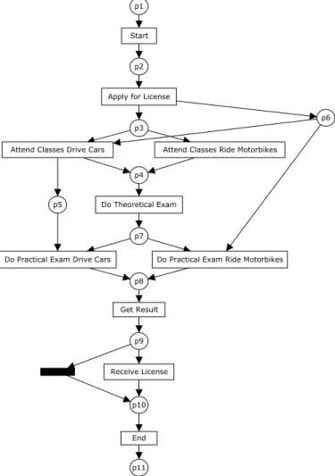
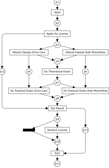
Drive Cars” and “Do Practical Exam Drive Cars”, and also between the tasks “Attend Classes Ride Motorbikes” and “Do Practical Exam Ride Motorbikes”. The dependency is non-local because it cannot be detected by simply looking at the direct predecessor and successor of those tasks in the log in Table 1, e.g. “Attend Classes Drive Cars” is never followed directly by “Do Practical Exam Drive Cars”. Moreover, note that only in some process instances (2 and 3) the task “Receive License” was executed. These process instances point to the cases in which the candidate passed the exams. Based on this log and these observations, process mining tools could be used to retrieve the model in Figure 2. In this case, we are using Petri nets [18,47] to depict this model. We do so because Petri nets will be used to explain the semantics of our internal representation. Moreover, we use Petri-net-based analysis techniques to analyse the resulting models. Using the Petri net representation, our tools allow for the automatic translation of the discovered model to a variety of modelling notations including Event-Driven Process Chains (used by ARIS, ARIS PPM, SAP) and YAWL (an open source workflow system).
Identifier Process instance
1 Start, Apply for License, Attend Classes Drive Cars,
Do Theoretical Exam, Do Practical Exam Drive Cars, Get Result, End
2 Start, Apply for License, Attend Classes Ride Motorbikes,
Do Theoretical Exam, Do Practical Exam Ride Motorbikes, Get Result, Receive License, End
3 Start, Apply for License, Attend Classes Drive Cars,
Do Theoretical Exam, Do Practical Exam Drive Cars, Get Result, Receive License, End
4 Start, Apply for License, Attend Classes Ride Motorbikes,
Do Theoretical Exam, Do Practical Exam Ride Motorbikes, Get Result, End
Table 1
Example of an event log with 4 process instances.
Petri nets are a formalism to model concurrent processes. Graphically, Petri
nets are bipartite directed graphs with two node types:places andtransitions.
Places represent conditions in the process. Transitions represent actions. Tasks in the event logs correspond to transitions in Petri nets. The state of a Petri net (or process for us) is described by adding tokens (black dots) to places.
The dynamics of the Petri net is determined by the firing rule. A transition
can be executed (i.e. an action can take place in the process) when all of its input places (i.e. pre-conditions) have at least a number of tokens that is equal to the number of directed arcs from the place to the transition. After execution, the transition removes tokens from the input places (one token is removed for every input arc from the place to the transition) and produces tokens for the output places (again, one token is produced for every output
arc). Besides, the Petri nets that we consider have a single start place and a
singleend place. This means that the processes we describe have a single start
point and a single end point. For the Petri net in Figure 2, in the initial state there is only one token in place “p1”. This implies that “Start” is the only transition that can be executed in the initial state. When “Start” executes (or fires), one token is removed from the place “p1” and one token is added to the place “p2”. In a similar way, the firing of “Apply for License” marks place “p3”. In this marking, “Attend Classes Drive Cars” or “Attend Classes Ride Motorbikes” can fire. If “Attend Classes Drive Cars” fires, it consumes the token in “p3” and produces one token for “p4” and another for “p5”. Note that, although the place “p5” has now one token, the transition “Do Practical
Apply for License
Attend Classes Ride Motorbikes Attend Classes Drive Cars
Do Theoretical Exam
Do Practical Exam Drive Cars Do Practical Exam Ride Motorbikes
Get Result Receive License Start End p10 p1 p2 p3 p5 p6 p4 p7 p8 p9 p11
Fig. 2. Mined net for the log in Table 1.
Exam Drive Cars” cannot fire yet because the place “p7” is not marked. The enabling and firing of transitions proceeds in a similar way until the place “p11” is marked.
1.2 Limitations of Current Approaches
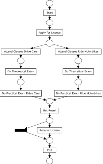
Current research in process mining [3,5,6,24,32,10,14,15,56,60] still has prob-lems to discover process models with certain structural constructs and/or to deal with the presence of noise in the logs (cf. Section 9). The main problem-atic constructs are: non-free-choice, invisible tasks and duplicate tasks [14].
Non-free-choice constructs combine synchronization and choice. The
exam-ple in Figure 2 illustrates a non-free-choice construct involving the tasks “Do Practical Exam Drive Cars” and “Do Practical Exam Ride Motorbikes”. The current techniques do not capture the dependency between (i) the tasks “At-tend Classes Drive Cars” and “Do Practical Exam Drive Cars”, and (ii) the
Apply for License
Attend Classes Ride Motorbikes Attend Classes Drive Cars
Do Theoretical Exam
Do Practical Exam Drive Cars Do Practical Exam Ride Motorbikes
Get Result
Receive License Start
End
Do Theoretical Exam
Fig. 3. Another model that correctly portraits the behavior in the log in Table 1.
Note that this model uses duplicate tasks instead of the non-free-choice construct
in Figure 2.
tasks “Attend Classes Ride Motorbikes” and “Do Practical Exam Ride
Motor-bikes”.Invisible tasks are only used for routing purposes and do not appear in
the log. For instance, the process in Figure 2 has an invisible task to skip the execution of the task “Receive License”. Current techniques have difficulties
discovering these routing tasks because they do not appear in the log.
Dupli-cate tasks means that multiple transitions have the same label in the original
process model. The problem here is that most of the mining techniques treat these duplicate tasks as a single one. For instance, Figure 3 shows a model that also captures the behavior in the log in Table 1 by duplicating the task
“Do Theoretical Exam”.Noise characterizes low-frequent behavior in the log.
It can appear in two situations: event traces were somehow incorrectly logged (for instance, due to temporary system misconfiguration) or event traces re-flect exceptional situations. Either way, most of the techniques will try to find a process model that can parse all the traces in the log. However, the presence of noise may hinder the correct mining of the most common behavior.
One of the reasons why the current techniques typically cannot cope with the above mentioned problematic constructs and/or with noisy logs is
be-cause their search is based on local information in the log. For instance, the
α-algorithm (see [5] for details) uses only information about which tasks
di-rectly succeed or precede one another in the process instances. As a result, this algorithm does not capture the dependency in non-free-choice constructs. For
example, the α-algorithm will never discover the Petri net in Figure 2, for the
log in Table 1, because none of the process instances has the sub-trace “At-tend Classes Drive Cars, Do Practical Exam Drive Cars” or “At“At-tend Classes Ride Motorbikes, Do Practical Exam Ride Motorbikes”. Consequently, the
α-algorithm will not link these tasks.
1.3 Genetic Process Mining
To overcome the limitations of the current process mining techniques, our
research uses genetic algorithms [21] to mine process models. The main
mo-tivation is to benefit from the global search that is performed by this kind of
algorithms.
Genetic algorithms are adaptive search methods that try to mimic the process of evolution. These algorithms start with an initial population of individuals. Every individual is assigned a fitness measure to indicate its quality. In our case, an individual is a possible process model and the fitness is a function that evaluates how well the individual is able to reproduce the behavior in the log. Populations evolve by selecting the fittest individuals and generating new
individuals using genetic operators such ascrossover (combining parts of two
or more individuals) andmutation (random modification of an individual).
When using genetic algorithms to mine process models, there are three main
concerns. The first is to define theinternal representation. The internal
sentation defines the search space of a genetic algorithm. The internal repre-sentation that we define and explain in this paper supports all the problematic
constructs, except for duplicate tasks. The second concern is to define the
fit-ness measure. In our case, the fitness measure evaluates the quality of a point
(individual or process model) in the search space against the event log. A ge-netic algorithm searches for individuals whose fitness is maximal. Thus, our fitness measure makes sure that individuals with a maximal fitness can parse all the process instances (traces) in the log and, ideally, not more than those traces. The reason for this is that we aim at discovering a process model that reflects as close as possible the behavior expressed in the event log. If the mined model allows for lots of extra behavior that cannot be derived from the log, it does not give a precise description of what is actually happening.
because they should ensure that all points in the search space defined by the internal representation may be reached when the genetic algorithm runs. This paper presents a genetic algorithm that addresses these three concerns.
1.4 Road Map
The remainder of the paper is organized as follows. Section 2 introduces the main definitions of Petri nets that are used in this paper. Section 3 explains the internal representation that we use and defines its semantics by mapping it onto Petri nets. Section 4 presents the genetic algorithm to mine processes that may have arbitrary mixtures of choice and synchronization (i.e., non-free-choice constructs) and invisible tasks. The genetic algorithm is also robust to noisy logs. Section 5 explains the metrics that we have developed to assess the quality of mined models while conducting the experiments. Section 6 discusses the experiments and results. The experiments include synthetic logs. Secion 7 shows the results of applying the genetic algorithm to logs from a municipality in The Netherlands. Section 8 compares the results of the genetic algorithm with the results obtained by two other related process mining techniques. Section 9 discusses the related work. Section 10 contains the conclusions and future work.
2 Preliminaries
This section introduces standard Petri-net notations that are used to explain the semantics of the internal representation of our genetic algorithm.
2.1 Petri Nets
We use a variant of the classic Petri-net model, namelyPlace/Transition nets.
For an elaborate introduction to Petri nets, the reader is referred to [18,47,52].
Definition 1 (P/T-nets) 2 A Place/Transition net, or simply P/T-net, is
a tuple (P, T, F) where:
(1) P is a finite set of places,
2 In the literature, the class of Petri nets introduced in Definition 2 is sometimes referred to as the class of (unlabeled)ordinary P/T-nets to distinguish it from the class of Petri nets that allows more than one arc between a place and a transition, and the class of Petri nets that allows for transition labels.
A
B
C D
E F
Fig. 4. An example of a Place/Transition net.
(2) T is a finite set of transitions such that P ∩T =∅, and
(3) F ⊆(P ×T)∪(T ×P) is a set of directed arcs, called the flow relation.
A marked P/T-net is a pair (N, s), where N = (P, T, F) is a P/T-net and
where s is a bag over P denoting the marking of the net, i.e. s ∈ P → IN.
The set of all marked P/T-nets is denoted N.
A marking is a bag over the set of places P, i.e., it is a function from P to
the natural numbers. We use square brackets for the enumeration of a bag,
e.g., [a2, b, c3] denotes the bag with two a-s, one b, and three c-s. The sum of
two bags (X +Y), the difference (X −Y), the presence of an element in a
bag (a∈X), the intersection of two bags (X∩Y) and the notion of subbags
(X ≤Y) are defined in a straightforward way and they can handle a mixture
of sets and bags.
LetN = (P, T, F) be a P/T-net. Elements of P ∪T are called nodes. A node
x is an input node of another node y iff there is a directed arc from x to y
(i.e., (x, y)∈F orxF y for short). Node x is an output node of y iff yF x. For
any x ∈P ∪T, N
•x ={y |yF x} and xN•={y |xF y}; the superscript N may
be omitted if clear from the context.
Figure 4 shows a P/T-net consisting of 7 places and 6 transitions. Transition
A has one input place and two output places. Transition A is an AND-split.
Transition D has two input places and one output place. Transition D is an
AND-join. The black dot in the input place ofAandE represents a token. This
token denotes the initial marking. The dynamic behavior of such a marked
P/T-net is defined by afiring rule.
Definition 2 (Firing rule) Let N = ((P, T, F), s) be a marked P/T-net.
Transition t ∈T is enabled, denoted (N, s)[ti, iff •t ≤s. The firing rule [ i
⊆ N ×T × N is the smallest relation satisfying for any(N = (P, T, F), s)∈
N and any t∈T, (N, s)[ti ⇒(N, s) [ti(N, s− •t+t•).
In the marking shown in Figure 4 (i.e., one token in the source place),
tran-sitions A and E are enabled. Although both are enabled only one can fire. If
transition A fires, a token is removed from its input place and tokens are put
in its output places. In the resulting marking, two transitions are enabled: B
inter-leaving semantics. In other words, parallel tasks are assumed to be executed in some order.
Definition 3 (Reachable markings) Let (N, s0) be a marked P/T-net in
N. A marking s is reachable from the initial marking s0 iff there exists a
sequence of enabled transitions whose firing leads from s0 to s. The set of
reachable markings of (N, s0) is denoted [N, s0i.
The marked P/T-net shown in Figure 4 has 6 reachable markings. Sometimes it is convenient to know the sequence of transitions that are fired in order to reach some given marking. This paper uses the following notations for
se-quences. LetAbe some alphabet of identifiers. Asequence of length n, for some
natural number n∈IN, over alphabet Ais a function σ:{0, . . . , n−1} →A.
The sequence of length zero is called the empty sequence and writtenε. For the
sake of readability, a sequence of positive length is usually written by
juxta-posing the function values. For example, a sequence σ={(0, a),(1, a),(2, b)},
for a, b ∈ A, is written aab. The set of all sequences of arbitrary length over
alphabetA is written A∗.
Definition 4 (Firing sequence) Let (N, s0) withN = (P, T, F)be a
mark-ed P/T net. A sequence σ ∈ T∗ is called a firing sequence of (N, s
0) if and
only if, for some natural number n ∈ IN, there exist markings s1, . . . , sn and
transitions t1, . . . , tn ∈T such that σ =t1. . . tn and, for all i with 0≤i < n,
(N, si)[ti+1i and si+1=si− •ti+1+ti+1•. (Note that n= 0 implies that σ =ε
and that ε is a firing sequence of (N, s0).) Sequence σ is said to be enabled in
marking s0, denoted (N, s0)[σi. Firing the sequenceσ results in a markingsn,
denoted (N, s0) [σi(N, sn).
For the marked Petri net shown in Figure 4, some possible firing sequences are
ABCD, ACBD and AE. Note that, for these firing sequences, the resulting
marking has a single token and this token is in the output place of transitions
D and F.
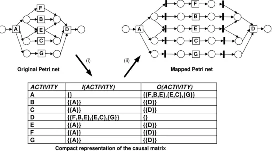
3 Internal Representation and Semantics
When defining the internal representation to be used by our genetic algorithm, the main requirement was that this representation should express the depen-dencies between the tasks in the log. In other words, the model should clearly express which tasks would enable the execution of other tasks. Additionally, it would be nice if the internal representation would be compatible with a formal-ism to which analysis techniques and tools exist. This way, these techniques could also be applied to the discovered models. Thus, one option would be to directly represent the individual (or process model) as a Petri net [18,47].
How-(ii) (i) A E B C D
Original Petri net Mapped Petri net
F G A F B C E G D
Compact representation of the causal matrix
ACTIVITY I(ACTIVITY) O(ACTIVITY)
A {} {{F,B,E},{E,C},{G}} B {{A}} {{D}} C {{A}} {{D}} D {{F,B,E},{E,C},{G}} {} E {{A}} {{D}} F {{A}} {{D}} G {{A}} {{D}}
Fig. 5. Mapping of a PN with more than one place between two tasks (or transitions).
ever, such a representation would require determining the number of places in every individual and this is not the core concern. It is more important to show the dependencies between the tasks and the semantics of the split/join tasks. Therefore, we defined an internal representation that is as expressive as Petri nets (from the task dependency perspective) but that only focuses
on the tasks. This representation is called causal matrix. Figure 5 illustrates
in (i) the causal matrix that expresses the same task dependencies that are in the “original Petri net”. The causal matrix shows which tasks enable the
execution of other tasks via the matching of input (I) and output (O)
con-dition functions. The sets returned by the concon-dition functions I and O have
subsets that contain the tasks in the model. Tasks in a same subset have
an XOR-split/join relation. Sets in different subsets have an AND-split/join
relation. Thus, everyI andO set expresses a conjunction of exclusive
disjunc-tions. Additionally, a task may appear in more than one subset in a same set.
As an example, for task D in the original Petri net in Figure 5 the causal
matrix states that I(D) ={{F, B, E},{E, C},{G}} because D is enabled by
an AND-join construct that has 3 places. From top to bottom, the first place
has a token whenever F or B or E fires. The second place, whenever E or
C fires. The third place, whenever G fires. Similarly, the causal matrix has
O(D) ={}because D is executed last in the model. The following definition
formally defines these notions.
Definition 5 (Causal Matrix) A Causal Matrix is a tuple CM = (A, C, I, O), where
- A is a finite set of activities,
- I :A→ P(P(A)) is the input condition function,3
- O :A→ P(P(A)) is the output condition function,
such that
- C ={(a1, a2)∈A×A | a1 ∈SI(a2)},4
- C ={(a1, a2)∈A×A | a2 ∈SO(a1)},
- C∪ {(ao, ai)∈A×A | ao
C
•=∅ ∧ C• ai =∅} is a strongly connected graph,
The set of all causal matrices is denoted byCM, and a bag of causal matrices
is denoted by CM[].
Any Petri net without duplicate tasks and without more than one place with the same input tasks and the same output tasks can be mapped to a causal matrix. Definition 6 formalizes such a mapping. The main idea is that there
is a causal relation C between any two tasks t and t0 whenever at least one
of the output places of t is an input place of t0. Additionally, the I and O
condition functions are based on the input and output places of the tasks. This is a natural way of mapping because the input and output places of Petri nets actually reflect the conjunction of disjunctions that these sets express.
Definition 6 (ΠP N→CM) Let PN = (P, T, F) be a Petri net. The mapping
of PN is a tuple ΠP N→CM(PN) = (A, C, I, O), where
- A=T,
- C ={(t1, t2)∈T ×T | t1• ∩ •t2 6=∅},
- I ∈T → P(P(T)) such that ∀t∈T I(t) ={•p | p∈ •t},
- O ∈T → P(P(T)) such that ∀t∈T O(t) ={p• | p∈t•}.
The semantics of the causal matrix can be easily understood by mapping them back to Petri nets. This mapping is formalized in Definition 7. Conceptually, the causal matrix behaves as a Petri net that contains visible and invisible tasks. For instance, see Figure 5. This figure shows (i) the mapping of a Petri net to a causal matrix and (ii) the mapping from the causal matrix to a Petri net. The firing rule for the mapped Petri net is very similar to the firing rule of Petri nets in general (cf. Definition 2). The only difference concerns the invisible tasks. Enabled invisible tasks can only fire if their firing enables a visible task. Similarly, a visible task is enabled if all of its input places have
tokens or if there exits a set of invisible tasks that are enabled and whose
firing will lead to the enabling of the visible task. Conceptually, the causal matrix keeps track of the distribution of tokens at a marking in the output places of the visible tasks. The invisible tasks can be seen as “channels” or “pipes” that are only used when a visible task needs to fire. Every causal 3 P(A) denotes the powerset of some setA.
4 S
matrix starts with a token at the start place. Finally, we point out that, in
Figure 5, although the mapped Petri net does not have the same structure
of the original Petri net, these two nets are behaviorally equivalent. In other
words, given that these two nets initially have a single token and this token
is at the start place (i.e., the input place of A), the set of traces the two nets
can generate is the same.
Definition 7 (ΠN
CM→P N) Let CM = (A, C, I, O) be a causal matrix. The
naive Petri net mapping of CM is a tuple ΠN
CM→P N = (P, T, F), where - P ={i, o} ∪ {it,s | t∈A ∧ s ∈I(t)} ∪ {ot,s | t ∈A ∧ s∈O(t)}, - T =A∪ {mt1,t2 | (t1, t2)∈C}, - F ={(i, t) | t ∈ A ∧ C • t =∅} ∪ {(t, o) | t ∈A ∧ t C•= ∅} ∪ {(it,s, t) | t ∈ A ∧ s ∈ I(t)} ∪ {(t, ot,s) | t ∈ A ∧ s ∈O(t)} ∪ {(ot1,s, mt1,t2) | (t1, t2) ∈ C ∧ s ∈O(t1) ∧ t2 ∈s}∪{(mt1,t2, it2,s)|(t1, t2)∈C ∧ s ∈I(t2) ∧ t1 ∈s}. Definition 7 shows a rather naive approach to generate the mapped Petri net shown in Figure 5. However, as shown in [16], there are special situations in which more sophisticated mappings are possible.
4 Genetic Algorithm
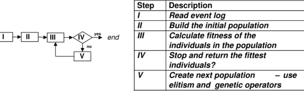
In this section we describe the main steps of our genetic algorithm. Figure 6 shows how they are related.
start I II III
V
IV yes end no
Step Description
I Read event log
II Build the initial population III Calculate fitness of the
individuals in the population IV Stop and return the fittest
individuals?
V Create next population – use elitism and genetic operators
Fig. 6. Main steps of our genetic algorithm.
4.1 Initial Population
The initial population is randomly built by the genetic algorithm. As explained in Section 3, individuals are causal matrices. When building the initial popu-lation, we ensure that the individuals comply with Definition 5. Given a log, all individuals in any population of the genetic algorithm have the same set
The setting of the causality relation C can be done via a completely random approach or a heuristic one. The random approach uses 50% probability for
establishing (or not) a causality relation between two task inA. The heuristic
approach uses the information in the log to determine the probability that two tasks are going to have a causality relation set. In a nutshell, the heuristics
works as follows: the more often a task t1 is directly followed by a task t2
(i.e. the subtrace “t1, t2” appears in traces in the log), the higher the
prob-ability that individuals are built with a causality relation from t1 to t2 (i.e.,
(t1, t2) ∈ C). This heuristic way of building an individual is based on the
work presented in [60]. Subsection 4.1.1 has more details about the heuristic approach. Once the causality relations of an individual are determined, the
condition functions I and O are randomly built. This is done by setting a
maximum size n for any input or output condition function set of a task t
in the initial population5. Every task t
1 that causally precedes a task t2, i.e.
(t1, t2) ∈ C, is randomly inserted in one or more subsets of the input
con-dition function of t2. A similar process is done to set the output condition
function of a task6. In our case, we set the number of distinct tasks in the log
as the maximum size for any input/output condition function set in the initial
population7. As a result, the initial population can have any individual in the
search space defined by a set of activities A, and that satisfy the constraints
for the size of the input/output condition function sets. Note that the higher the amount of tasks that a log contains, the bigger this search space. Finally, we emphasize that no further limitations to the input/output condition func-tions sets are made in the other steps of the genetic algorithm. Therefore, during the “Step V” in the Figure 6, these sets can increase or shrink as the population evolves.
4.1.1 Heuristics to Build the Causality Relation of a Causal Matrix
When applying a genetic algorithm to a domain, it is common practice to “give a hand” to the genetic algorithm by using well-know heuristics (in this domain) to build the initial population [21]. Studies show that the use of heuristics often does not alter the end result (if the genetic algorithm runs for infinite amount of time), but it may speed the early stages of the evolution.
The GAs that use heuristics are called hybrid genetic algorithms.
In our specific domain - process mining - some heuristics have proven to give reasonable solutions when used to mine event logs. These heuristics are mostly based on local information in the event-log. Due to its similarities to other related work, we use the heuristics in [60] to guide the setting of the causality
5 Formally: ∀ t∈A[|I(t)| ≤n ∧ |O(t)| ≤n]. 6 Formally: ∀ t1,t2∈A,(t1,t2)∈C[∃i ∈ I(t2) : t1 ∈ i] and ∀t1,t2∈A,(t1,t2)∈C[∃o ∈ O(t1) : t2∈o]. 7 Formally: ∀ t∈A[|I(t)| ≤ |A| ∧ |O(t)| ≤ |A|].
relations in the individuals of the initial population. These heuristics are based
on thedependency measure. To define this measure, we first need to formalize
the notion of an event log.
Definition 8 (Event Trace, Event Log) LetT be a set of tasks. σ∈T∗ is
an event trace and L :T∗ → IN is an event log. For any σ ∈ dom(L), L(σ)
is the number of occurrences of σ. The set of all event logs is denotes by L.
Note that we use dom(f) and rng(f) to respectively denote the domain and
range of a function f. Furthermore, we use the notation σ ∈ L to denote
σ ∈ dom(L)∧L(σ) ≥ 1. For example, assume a log L = [abcd, acbd, abcd]
for the net in Figure 4. Then, we have that L(abcd) = 2, L(acbd) = 1 and
L(ab) = 0.
The dependency measure basically indicates how strongly a task depends (or
is caused) by another task. The more often a taskt1 directly precedes another
task t2 in the log, and the less often t2 directly precedes t1, the stronger is
the dependency between t1 and t2. In other words, the more likely it is that
t1 is a cause to t2. The dependency measure is given in Definition 9. The
notation used in this definition is as follows.l2l :T ×T× L →IN is a function
that detects length-two loops.l2l gives the number of times that the substring
“t1t2t1” occurs in the logL.follows :T×T×L →IN is a function that returns
the number of times that a task is directly followed by another one. That is,
how often the substring “t1t2” occurs in the log L.
Definition 9 (Dependency Measure - D ) Let L be an event log. Let T
be the set of tasks in L. Let t1 and t2 be two tasks in T. The dependency
measure D:T ×T × L →IR is a function defined as:
D(t1, t2, L) = l2l(t1,t2,L)+l2l(t2,t1,L) l2l(t1,t2,L)+l2l(t2,t1,L)+1 if t1 6=t2 and l2l(t1, t2, L)>0, follows(t1,t2,L)−follows(t2,t1,L)
follows(t1,t2,L)+follows(t2,t1,L)+1 if t1 6=t2 and l2l(t1, t2, L) = 0,
follows(t1,t2,L)
follows(t1,t2,L)+1 if t1 =t2.
Observe that the dependency relation distinguishes between tasks in short loops (length-one and length-two loops) and tasks in parallel. Moreover, the “+1” in the denominator is used to benefit more frequent observations over
less frequent ones. For instance, if a length-one-loop “tt” happens only once
in the log L, the dependency measure D(t, t, L) = 0.5. However, if this same
length-one-loop would occur a hundred times in the log, D(t, t, L) = 0.99.
Thus, the more often a substring (or pattern) happens in the log, the stronger the dependency measure.
Once the dependency relations are set for the input event log, the genetic algorithm uses it to randomly build the causality relations for every individual in the initial population. The pseudo-code for this procedure is the following: Pseudo-code:
input: An event-log L, a power value p, the dependency function D.
output: A causality relation C.
(1) T ←−set of tasks in L.
(2) C ←− ∅.
(3) FOR every tuple (t1, t2) in T ×T do:
(a) Randomly select a numberrbetween 0 (inclusive) and 1.0 (exclusive).
(b) IF r < D(t1, t2, L)p then: (i) C ←−C∪ {(t1, t2)}.
(4) Return the causality relationC.
Note that we use a power valuepto control the “influence” of the dependency
measure in the probability of setting a causality relation. Higher values for p
lead to the inference of fewer causality relations among the tasks in the event log, and vice-versa.
4.2 Fitness Calculation
As discussed in Section 1, process mining aims at discovering a process model from an event log. This mined process model should give a good insight about what the behavior in the log is. In other words, the mined process model
should becomplete and precise from a behavioral perspective. A process model
is complete when it can parse (or reproduce) all the event traces in the log. A process model is precise when it cannot parse more than the traces in the log. The requirement that the mined model should also be precise is important because different models are able to parse all event traces and these models may allow for extra behavior that does not belong to the log. To illustrate this we consider the nets shown in Figure 7. These models can also parse the traces in Table 1, but they allow for extra behavior. For instance, both models allow for the applicant to take the exam before attending to classes. The fitness function guides the search process of the genetic algorithm. Thus, the fitness of an individual is assessed by benefiting the individuals that can parse more event traces in the log (the “completeness” requirement) and by punishing the individuals that allow for more extra behavior than the one expressed in the log (the “preciseness” requirement).
To facilitate the explanation of our fitness measure, we divide it into three parts. First, we discuss in Subsection 4.2.1 how we defined the part of the fitness measure that guides the genetic algorithm towards individuals that are
Attend Classes Ride Motorbikes Attend Classes
Drive Cars Do Theoretical Exam Do Practical
Exam Drive Cars Do Practical Exam Ride Motorbikes Get Result LicenseReceive Start
End
Start Apply for License
Do Practical Exam Drive Cars
Do Practical Exam Ride Motorbikes Get Result Attend Classes Drive Cars Attend Classes Ride Motorbikes Do Theoretical Exam Receive License End
Apply for License (a)
(b)
Fig. 7. Example of nets that can also reproduce the behavior for the log in Table 1. The problem here is that these nets allow for extra behavior that is not in the log. more complete. Second, we show in Subsection 4.2.2 how we defined the part of the fitness measure that benefits individuals that are more precise. Finally, we show in Subsection 4.2.3 the fitness measure that our genetic algorithm is using. This fitness measure combines the partial fitness measures that are presented in the subsections 4.2.1 and 4.2.2.
4.2.1 The “Completeness” Requirement
The “completeness” requirement of our fitness measure is based on the pars-ing of event traces by individuals. For a noise-free log, the perfect individual should have fitness 1. This means that this individual could parse all the traces in the log. Therefore, a natural fitness for an individual to a given
log seems to be the number of properly parsed event traces8 divided by the
total number of event traces. However, this fitness measure is too coarse be-cause it does not give an indication about (i) how many parts of an individual are correct when the individual does not properly parse an event trace and 8 An event trace is properly parsed by an individual if, for an initial marking that contains a single token and this token is at the start place of the mapped Petri net for this individual, after firing the visible tasks in the order in which they appear in the event trace, the end place is the only one to be marked and it has a single token.
(ii) the semantics of the split/join tasks. For instance, if a net has an AND-split instead of an XOR-AND-split, it may happen that all tasks in a trace can be replayed by this net, but this net does not proper complete for this trace because tokens remain at some of the output places of the AND-split task. So, we defined a more elaborate fitness function: when the task to be parsed is not enabled, the problems (e.g. number of missing tokens to enable this task) are registered and the parsing proceeds as if this task would be
en-abled. This continuous parsing semantics is more robust because it gives a
better indication of how many tasks do or do not have problems during the parsing of a trace. The partial fitness function that tackles the “complete-ness” requirement is in Definition 10. The notation used in this definition
is as follows. allParsedActivities(L, CM) gives the total number of tasks in
the event log L that could be parsed without problems by the causal
ma-trix (or individual)CM.numActivitiesLog(L) gives the number of tasks inL.
allMissingTokens(L, CM) indicates the number of missing tokens in all event
traces.allExtraTokensLeftBehind(L, CM) indicates the number of tokens that
were not consumed after the parsing has stopped plus the number of tokens
of the end place minus 1 (because of proper completion). numTracesLog(L)
indicates the number of traces in L. numTracesMissingTokens(L, CM) and
numTracesExtraTokensLeftBehind(L, CM) respectively indicate the number
of traces in which tokens were missing and tokens were left behind during the parsing.
Definition 10 (Partial Fitness - PFcomplete ) Let L be a non-empty event
log. LetCM be a causal matrix. Then the partial fitness PFcomplete :L × CM →
(−∞,1] is a function defined as:
PFcomplete(L, CM) = allParsedActivities(L, CM)−punishment numActivitiesLog(L) where punishment = allMissingTokens(L, CM) numTracesLog(L)−numTracesMissingTokens(L, CM) + 1 + allExtraTokensLeftBehind(L, CM) numTracesLog(L)−numTracesExtraTokensLeftBehind(L, CM) + 1
The partial fitness PFcomplete gives a more detailed indication about how fit
an individual is to a given log. The function allMissingTokens penalizes (i)
nets with XOR-split where it should be an AND-split and (ii) nets with an
AND-join where it should be an XOR-join. Similarly, the function
XOR-split and (ii) nets with an XOR-join where it should be an AND-join. Note
that we weigh the impact of theallMissingTokens and
allExtraTokensLeftBe-hind functions by respectively dividing them by the number of event traces
minus the number of event traces with missing and left-behind tokens. The main idea is to promote individuals that correctly parse the more frequent
behavior in the log. Additionally, if two individuals have the samepunishment
value, the one that can parse more tasks has a better fitness because its miss-ing and left-behind tokens impact fewer tasks. This may indicate that this
individual has more correctI and O condition functions than incorrect ones.
In other words, this individual is a better candidate to produce offsprings for the next population (see Subsection 4.4).
4.2.2 The “Preciseness” requirement
The “preciseness” requirement is based on discovering how much extra be-havior an individual allows for. To define a fitness measure to punish models that express more than it is in the log is especially difficult because we do not have negative examples to guide our search. Note that the event logs show the allowed (positive) behavior, but they do not express the forbidden (negative) one.
One possible solution to punish an individual that allows for undesirable
be-havior could be to build the coverability graph [47] of the mapped Petri net
for this individual and check the fraction of event traces this individual can generate that are not in the log. The traces that express different paths of execution for parallelism are not considered as extra behavior. The main idea in this approach is to punish the individual for every extra event trace it gen-erates. Unfortunately, building the coverability graph is not very practical and it is unrealistic to assume that all possible behavior is present in the log. Because proving that a certain individual is precise is not practical, we use a simpler solution to guide our genetic algorithm towards solutions that have
“less extra behavior”. We check, for every marking, thenumber of visible tasks
that are enabled. Individuals that allow for extra behavior tend to have more
enabled tasks than individuals that do not. For instance, the nets in Fig-ure 7 have more enabled tasks in most reachable markings than the net in Figure 2. The main idea in this approach is to benefit individuals that have a smaller amount of enabled tasks during the parsing of the log. This is the
measure we use to define our second partial fitness function PFprecise that is
presented in Definition 11. The notation used in this definition is as follows.
allEnabledActivities(L, CM) indicates the number of activities that were
en-abled during the parsing of the logLby the causal matrix (or individual)CM.
allEnabledActivities(L, CM[]) apply allEnabledActivities(L, CM) (see
population) CM[]. The function max(allEnabledActivities(L,CM[])) returns
the maximum value of the amount of enabled tasks that individuals in the
given population (CM[]) had while parsing the log (L).
Definition 11 (Partial Fitness - PFprecise) LetLbe a non-empty event log.
LetCM be a causal matrix. LetCM[]be a bag of causal matrices that contains
CM. The partial fitness PFprecise :L × CM × CM[]→[0,1]is a function
de-fined as
PFprecise(L, CM, CM[]) =
allEnabledActivities(L, CM)
max(allEnabledActivities(L,CM[]))
The partial fitness PFprecise gives an indication of how much extra behavior
an individual allows for in comparison to other individuals in the same
pop-ulation. The smaller thePFprecise of an individual is, the better. This way we
avoid over-generalizations.
4.2.3 Fitness - Combining the “Completeness” and “Preciseness” Require-ments
While defining the fitness measure, we decided that the “completeness” re-quirement should be more relevant than the “preciseness” one. The reason is that we are only interested in precise models that are also complete. The resulting fitness is defined as follows.
Definition 12 (Fitness - F) Let L be a non-empty event log. Let CM be
a causal matrix. Let CM[] be a bag of causal matrices that contains CM.
Let PFcomplete and PFprecise be the respective partial fitness functions given in
definitions 10 and 11. Let κ be a real number greater than 0 and smaller or
equal to1 (i.e., κ∈(0,1]). Then the fitness F :L × CM × CM[]→ (−∞,1)
is a function defined as
F(L, CM, CM[]) =PFcomplete(L, CM)−κ∗PFprecise(L, CM, CM[])
The fitness F weighs (by κ) the punishment for extra behavior. Thus, if a
set of individuals can parse all the traces in the log, the one that allows for less extra behavior will have a higher fitness value. For instance, assume a population with the corresponding individual for the net in Figure 2 and the
corresponding individuals for the nets in Figure 7. If we calculate the fitnessF
of these three individuals with respect to the log in Table 1, the individual in Figure 2 will have the highest fitness value among the three and the individual in Figure 7(b), the lowest fitness value.
4.3 Stop Criteria
The mining algorithm stops when (i) it computesngenerations, wherenis the
maximum number of generations that is allowed; or (ii) the fittest individual
has not changed for n/2 generations in a row.
4.4 Genetic Operators
We use elitism, crossover and mutation to build the individuals of the next
generation. A percentage of the best individuals (the elite) is directly copied
to the next population. The other individuals in the population are generated via crossover and mutation. Two parents produce two offsprings. To select one
parent, atournament is played in which five individuals in the population are
randomly drawn and the fittest one always wins. The crossover and mutation operator are explained respectively in subsections 4.4.1 and 4.4.2.
4.4.1 Crossover
Crossover is a genetic operator that aims at recombining existing material in the current population. In our case, this material is the current causality relations (cf. Definition 5) in the population. Thus, the crossover operator used by our genetic algorithm should allow for the complete search of the space defined by the existing causality relation in a population. Given a set of causality relations, the search space contains all the individuals that can be created by any combination of a subset of the causality relations in the population. Thus, our crossover operator allows an individual to: lose tasks
from the subsets in its I/O condition functions (but not necessarily causality
relations because a same task may be in more than one subset of an I/O
condition function), add tasks to the subsets in its I/O condition functions
(again, not necessarily causality relations), exchange causality relations with other individuals, incorporate causality relations that are in the population but are not in the individual, lose causality relations, decrease the number of
subsets in itsI/O condition functions, and/or increase the number of subsets
in its I/O condition functions. The crossover rate determines the probability
that two parents undergo crossover. The crossover point of two parents is a randomly chosen task. The pseudo-code for the crossover operator is as follows: Pseudo-code:
input: Two parents (parent1 and parent2), crossover rate.
output: Two possibly recombined offsprings (offspring1 and offspring2).
(2) With probability “crossover rate” do:
(a) Randomly select a task t to be the crossover point of the offsprings.
(b) Randomly select a swap point sp1 for I1(t) 9. The swap point goes
from position 0 to n−1, where n is the number of subsets in the
condition function I1(t).
(c) Randomly select a swap pointsp2 for I2(t).
(d) remainingSet1(t) equals subsets in I1(t) that are between position 0
and sp1 (exclusive).
(e) swapSet1(t) equals subsets in I1(t) whose position equals or bigger
than sp1.
(f) Repeat steps 2d and 2e but respectively use remainingSet2(t), I2(t),
sp2 and swapSet2(t) instead of remainingSet1(t), I1(t),sp1 and
swapSet1(t).
(g) FOR every subset S2 in swapSet2(t) do:
(i) With equal probability perform one of the following steps:
(A) Add S2 as a new subset in remainingSet1(t).
(B) Join S2 with an existing subset X1 in remainingSet1(t).
(C) Select a subset X1 in remainingSet1(t), remove the
ele-ments ofX1 that are also inS2 and addS2 toremaining−
Set1(t).
(h) Repeat Step 2g but respectively useS1,swapSet1(t),X2andremain−
ingSet2(t) instead of S2, swapSet2(t),X1 and remainingSet1(t).
(i) I1(t)←−remainingSet1(t) and I2(t)←−remainingSet2(t).
(j) Repeat steps 2b to 2h but use O(t) instead of theI(t).
(k) Update the related tasks to t.
(3) Return offspring1 and offspring2.
Note that, after crossover, the number of causality relations for the whole population remains constant, but how these relations appear in the offsprings may be different from the parents. Moreover, the offsprings may be differ-ent even when both pardiffer-ents are equal. For instance, consider the situation in which the crossover operator receives as input two parents that are equal to the causal matrix in Figure 5. Assume that (i) the crossover point is
the task D, (ii) we are doing crossover over the input condition function
I(D) = {{F, B, E},{E, C},{G}}, and (iii) the swap points are sp1 = 1
and sp2 = 2. Then, we have that the remainingSet1(D) = {{F, B, E}}, the
swapSet1(D) = {{E, C},{G}}, theremainingSet2(D) ={{F, B, E},{E, C}},
theswapSet2(D) = {{G}}. Let us first crossover the subsets in theswapSet2(D)
with the remainingSet1(D). During the crossover, the genetic algorithm
ran-domly chooses to merge the subset S2 = {G} in the swapSet2(D) with the
existing subset X1 ={F, B, E}. In a similar way, while swapping the subsets
9 We use the notation I
j(t) to get the subset returned by the input condition
function I of task t in individual j. In this pseudo-code, the individuals are the
in swapSet1(D) with the remainingSet2(D), the algorithm randomly chooses
(i) to insert the subset S1 = {E, C} and remove task E from the subset
X2 = {F, B, E}, and (ii) to insert the subset S1 = {G} as a new subset
in the remainingSet2(D). The result is that I1(D) = {{F, B, E, G}}} and
I2(D) = {{F, B},{E, C},{G}}. The output condition functions O1(D) and
O2(D) do not change after the crossover operator because the taskDdoes not
have any output task. After the crossover, the mutation operator takes place.
4.4.2 Mutation
The mutation operator aims at inserting new material in the current pop-ulation. In our case, this means that the mutation operator may change the existing causality relations of a population. Thus, our mutation
oper-ator performs one of the following actions to the I/O condition functions
of a task in an individual: (i) randomly choose a subset and add a task
(in A) to this subset, (ii) randomly choose a subset and remove a task out
of this subset, or (iii) randomly redistribute the elements in the subsets of
I/O into new subsets. For example, consider the input condition function
of task D in Figure 5. I(D) = {{F, B, E},{E, C},{G}} can be mutated to
(i) {{F, B, E},{E, C},{G, D}} if task D is added to the subset {G}, (ii)
{{F, B, E},{C},{G}} if task E is removed from the subset {E, C}, or (iii)
{{F},{E, C, B},{G},{E}} if the elements in the originalI(D) are randomly
redistributed in a randomly chosen number of new subsets. Every task in an offspring may undergo mutation with the probability determined by the
mutation rate. The pseudo-code for the mutation operator is as follows:
Pseudo-code:
input: An individual, mutation rate.
output: A possibly mutated individual.
(1) For every taskt in the individual do:
(a) With probabilitymutation rate do one of the following operations for
the condition function I(t):
(i) Select a subsetX inI(t) and add a taskt0 toX, wheret0 belongs
to the set of tasks in the individual.
(ii) Select a subset X in I(t) and remove a task t0 from X, where
t0 belongs to X. If X is empty after t0 removal, exclude X from
I(t).
(iii) Redistribute the elements in I(t). 10
(b) Repeat Step 1a, but use the condition function O(t) instead of I(t).
10Details about this step: (i) Get a list with the elements ofI(t); (ii) Create nsets (n is the number of elements in I(t)) and randomly distribute them in the n sets; and (iii) Filter out the non-empty sets. These non-empty sets are now the subsets ofI(t).
(c) Update the related tasks to t.
As the reader may already have noticed, both the crossover and the mutation operators perform a repairing operation at the end of their executions. The “update the related tasks” operation makes sure that the individual is still compliant with the Definition 5 after undergoing crossover and/or mutation.
5 Analysis Metrics
The genetic algorithm searches for models that arecomplete and precise (see
Subsection 4.2). Therefore, when evaluating the results of our experiments, we should check if the mined models are indeed complete and precise. At first sight, the natural way to check for this seemed to be to compare the causal matrix of the original model (the one that was simulated to created the synthetic event logs) with the causal matrix of the individual that was mined by the genetic algorithm. However, this is not a good evaluation criterion because there are different ways to model the exact behavior expressed in a log. For instance, consider the net in Figure 8. This net produces exactly the same behavior as the one in Figure 2. However, their causal matrices are different. Furthermore, even when the mined models are not complete and/or precise, we should be able to assess how much correct material they contain. This is important because we do not let the genetic algorithm run for an “infinite” amount of time. Thus, even when the mined model is not complete and precise, it is important to know if the genetic algorithm is going in the right direction.
In our experiments, we have three elements: (i) theoriginal model that is used
to build the synthetic event log, (ii) the syntheticevent log itself, and (iii) the
mined model (or individual). Thus, to analyse our results, we have defined
metrics that are based on two or more of these elements.
Checking for Completeness
To check for completeness, we only need the event log and the mined model. Recall that a model is complete when it can parse all the traces in the log without having missing tokens or tokens left behind. So, completeness can be
verified by calculating the partial fitnessP Fcomplete (see Definition 10) for the
event log and the mined model. Whenever P Fcomplete = 1, the mined model
is complete. Moreover, even when the mined model has P Fcomplete < 1, this
measure gives an indication of the quality of the mined model with respect to completeness.
Apply for License
Attend Classes Ride Motorbikes Attend Classes Drive Cars
Do Theoretical Exam
Do Practical Exam Drive Cars Do Practical Exam Ride Motorbikes
Get Result Receive License Start End p10 p1 p2 p3 p5 p6 p4 p7 p8 p9 p11
Fig. 8. Other mined net for the log in Table 1. Note that this net is behaviorally equivalent to the net in Figure 2, although they are structurally different. Note that the place “p6” has different input and output tasks in the two nets.
To check for preciseness, we need the original model, the event log and the
mined model11. The main reason why we could not define metrics only based
on the event log and the mined model, or the original model and the mined model, is because it is unrealistic to assume that the event log has all the possible traces that the original model can generate. In other words, it is unrealistic to assume that the log contains all possible event traces. Recall that a model is precise when it does not allow for more behavior than the one expressed in the log. Thus, if the log would be exhaustive, a possible metric to check for this preciseness could be to divide the number of traces that are in the log and that the mined model can generate by the amount of traces that the mined model can generate. Clearly, a precise mined model could not
11Note that in reality we do not know the original (or initial) model. However,
the only way to evaluate our results is to assume an initial model. Without an initial model, it is impossible to judge preciseness. In other words, there could be over-fitting or over-generalization, but it would be impossible to judge this.
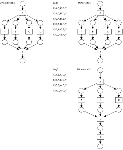
A B C A D y x y X D B C X A B C D Y OriginalModel Log1 X,A,B,C,D,Y X,A,C,B,D,Y X,C,A,D,B,Y X,B,A,D,C,Y X,D,A,C,B,Y X,C,D,B,A,Y Log2 X,A,B,C,D,Y X,B,A,C,D,Y X,C,B,A,D,Y X,B,C,A,D,Y MineModel1 MineModel2
Fig. 9. Example of two mined models that are complete and precise with respect to the logs, but both mined models can generate more traces than the ones in the log. Additionally, the coverability graph of the “MinedModel2” is different from the one of the “OriginalModel”.
generate more traces than the ones in the log. Note that this metric would be based on the event log and the mined model. Furthermore, metrics based on the mined and original models would also be possible if the log would be entire. For instance, we could compare the coverability graphs [47] of mapped Petri nets of the mined and the original models. In this case, the mined model would be precise whenever the coverability graphs would be equal. Note that sophisticated notions such as bisimulation [41] and branching bisimulation [22] could also be used. However, none of these metrics are suitable because in real-life applications the log does not hold all possible traces.
For instance, consider the situation illustrated in Figure 9. This figure shows the original model (“OriginalModel”), two synthetic logs (“Log1” and “Log2”) and their respective mined models (“MinedModel1” and “MinedModel2”).
“Log1” shows that the tasks A, B, C and D are (i) always executed after the
taskX and before the taskY and (ii) independent of each other. Thus, we can
in the “Log1”. However, note that the “MinedModel1”, although precise, can generate more traces than the ones in the “Log1”. A similar reasoning can be done for the “Log2” and the “MinedModel2”. Moreover, the coverability graph of the “MinedModel2” is different from the one of the “OriginalModel”. Actually, based on “Log2”, the “MinedModel2” is more precise than the “Orig-inalModel”. This illustrates that, when assessing how close the behavior of the mined and original models are, we have to consider the event log that was used by the genetic algorithm. Therefore, we have defined two metrics to quantify
how similar the behavior of the original model and the mined model arebased
on the event log used during the mining process.
The two metrics are the behavioral precision (BP) and the behavioral recall
(BR). Both metrics are based on the parsing of an event log by the mined
model and by the original model. The BP and BR metrics are respectively
formalized in definitions 13 and 14. These metrics basically work by checking, for the continuous semantics parsing of every task in every process instance of the event log, how many tasks are enabled in the mined model and how many are enabled in the original model. The more enabled tasks the models have in common, the more similar their behaviors are with respect to the event
log. The behavioral precisionBP checks how much behavior is allowed by the
mined model that is not by the original model. The behavioral recallBRchecks
for the opposite. Additionally, both metrics take into account how often a trace occurs in the log. This is especially important when dealing with logs in which some paths are more likely than others, because deviations corresponding the infrequent paths are less important than deviations corresponding to frequent behavior. Note that, assuming a log generated from an original model and a
mined model for this log, we can say that the closer their BP and BR are to
1, the more similar their behaviors. More specifically, we can say that:
- The mined model is as precise as the original model whenever BP and BR
are equal to 1. This is exactly the situation illustrated in Figure 9 for the “OriginalModel”, the “Log1” and the “MinedModel1”.
- The mined model ismore precise than the original model whenever BP = 1
and BR < 1. For instance, see the situation illustrated in Figure 9 for the
“OriginalModel”, the “Log2” and the “MinedModel2”.
- The mined model is less precise than the original model whenever BP <1
andBR = 1. For instance, see the situation illustrated for the original model
in Figure 2, the log in Figure 1, and the mined models in Figure 7.
Definition 13 (Behavioral Precision - BP) 12 Let L be an event log. Let
CMo and CMm be the respective causal matrices for the original (or base)
12For both definitions 13 and 14, whenever the denominator “|Enabled(CM, σ, i)|” is equal to 0, the whole division is equal to 0. For simplicity reasons, we have omitted this condition from the formulae.
model and for the mined one. Then the behavioral precision BP : L × CM ×
CM →[0,1] is a function defined as:
BP(L,CMo,CMm) = X σ∈L L(σ) |σ| × |σ| X i=1 |Enabled(CMo, σ, i)TEnabled(CMm, σ, i)| |Enabled(CMm, σ, i)| ! X σ∈L L(σ) where
- Enabled(CM, σ, i) gives the enabled activities at the causal matrix CM just
before the parsing of the element at position i in the trace σ. During the
parsing a continuous semantics is used (see Section 4.2.1).
Definition 14 (Behavioral Recall - BR) Let L be an event log. Let CMo
and CMmbe the respective causal matrices for the original (or base) model and
for the mined one. Then the behavioral recall BR :L × CM × CM →[0,1] is
a function defined as:
BR(L,CMo,CMm) = X σ∈L L(σ) |σ| × |σ| X i=1 |Enabled(CMo, σ, i)TEnabled(CMm, σ, i)| |Enabled(CMo, σ, i)| ! X σ∈L L(σ)
Reasoning about the Quality of the Mined Models
When evaluating the quality of a data mining approach (genetic or not), it is common to check if the approach tends to find over-general or over-specific solutions. In our case, the over-general solution is the one that can parse any trace that can be formed from the tasks in a log. This solution has a self-loop for every task in the log. The over-specific solution is the one that has a branch
for every unique trace in the log. Figure 10 illustrates an over-general and an
over-specific solution for the log in Table 1.
The over-general solution does belong to the search space considered in this
paper. However, this kind of solution can be easily detected by the metrics we
have defined so far. Note that, for a given original modelCMo, a logL
gener-ated by simulating CMo, and the mined over-general model CMm, it always
holds that: (i) the over-general model is complete (i.e.,P Fcomplete(L,CMm) =
1); (ii) while parsing the traces, all the tasks that are enabled in the original
Start Apply for License
Do Practical Exam Drive Cars
Do Practical Exam Ride Motorbikes Get Result Attend Classes Drive Cars Attend Classes Ride Motorbikes Do Theoretical Exam Receive License End
Start Start Start Start
Apply for License Apply for License Apply for License Apply for License
Attend Classes
Drive Cars Attend Classes Drive Cars Ride MotorbikesAttend Classes Ride MotorbikesAttend Classes
Do Theoretical
Exam Do Theoretical Exam Do Theoretical Exam Do Theoretical Exam
Do Practical Exam Drive Cars Do Practical
Exam Drive Cars Do Practical Exam Ride Motorbikes Do Practical Exam Ride Motorbikes
Get Result Get Result Get Result Get Result
Receive
License LicenseReceive
End
End End End
(a)
(b)
Fig. 10. Example of nets that are (a) over-general and (b) over-specific for the log in the Table 1.
1); and (iii) while parsing the traces, all the tasks of the over-general model are always enabled, i.e., the formula of the behavioral precision (see Definition 13) can be simplified to the formula in Equation 1. These three remarks are used
to detect over-general mined models during the experiments analysis. BP(L,CMo,CMm) = X σ∈L L(σ) |σ| × |σ| X i=1 |Enabled(CMo, σ, i)| |Am| ! X σ∈L L(σ) (1)
Contrary to the over-general solution, the over-specific one does not belong
to our search space because our internal representation (the causal matrix) does not support duplicate tasks. However, because our fitness only looks for the complete and precise behavior (not the minimal representation, like the
works on Minimal Description Length (MDL) [28]), it is still important to
check how similar the structures of the mined model and the original one are. Differences in the structure may point out another good solution or an overly complex solution. For instance, have a look at the model in Figure 11. This net is complete and precise from a behavioral point of view, but it contains extra unnecessary places. Note that the places “p12” and “p13” could be removed from the net without changing its behavior. In other words, “p12” and “p13” are implicit places [5]. Actually, because the places do not affect the net behavior, all the nets in figures 2, 8 and 11 have the same fitness. However, a metric that checks the structure of a net would, for instance, point out that the net in Figure 11 is a “superstructure” of the net in Figure 2, and has many elements in common with the net in Figure 8. So, even when we know that the over-specific solution is out of the search space defined in this paper, it is interesting to get a feeling about the structure of the mined models. That is why we developed two metrics to assess how much the mined
and original model have in common from a structural point of view.
The two metrics are the structural precision (SP) and the structural recall
(SR). Both metrics are based on thecausality relations of the mined and
orig-inal models, and were adapted from the precision and recall metrics presented
in [49]. The SP and SR metrics are respectively formalized in definitions 13
and 16. These metrics basically work by checking how many causality rela-tions the mined and the original models have in common. The more causality relations the two models have in common, the more similar their structures are. The structural precision assess how many causality relations the mined model has that are not in the original model. The structural recall works the other way around. Note that the structural similarity performed by these metrics does not consider the semantics of the split/join points. We have done so because the causality relations are the core of our genetic material (see Subsection 4.4). The semantics of the split/join tasks can only be correctly captured if the right dependencies (or causality relations) between the tasks in the log are also in place.
Apply for License
Attend Classes Ride Motorbikes Attend Classes Drive Cars
Do Theoretical Exam
Do Practical Exam Drive Cars Do Practical Exam Ride Motorbikes
Get Result Receive License Start End p10 p1 p2 p3 p5 p6 p4 p7 p8 p9 p11 p12 p13
Fig. 11. Example of a net that that is behavioral precise and complete w.r.t. the log in the Table 1, but that contains extra unnecessary (implicit) places (p12 and p13).
Definition 15 (Structural Precision - SP) 13 Let CMo and CMm be the
respective causal matrices for the original and the mined models. The structural
precision SP :CM × CM →[0,1] is a function defined as:
SP(CMo,CMm) =
|Co∩Cm|
|Cm|
Definition 16 (Structural Recall - SR) Let CMo and CMm be the
respec-tive causal matrices for the original and the mined model. The structural recall
13For both definitions 13 and 16, whenever the denominator “|C|” is equal to 0, the whole division is equal to 0. For simplicity reasons, we have omitted this condition from the formulae.