Analysis of ordinal data with cumulative link models estimation with the R-package ordinal

(1)

Analysis of ordinal data with cumulative link models —

estimation with the

R

_-package

ordinal

Rune Haubo B Christensen

(2)

1 Introduction

Ordered categorical data, or simplyordinal data, are commonplace in scientific disciplines where humans are used as measurement instruments. Examples include school gradings, ratings of preference in consumer studies, degree of tumor involvement in MR images and animal fitness in field ecology. Cumulative link models are a powerful model class for such data since observations are treated rightfully as categorical, the ordered nature is exploited and the flexible regression framework allows in-depth analyses.

The namecumulative link models is adopted from Agresti (2002), but the models are also known as ordinal regression models although that term is sometimes also used for other regression models for ordinal responses such ascontinuation ratio models (see e.g., Agresti, 2002). Other aliases areordered logit modelsandordered probit models(Greene and Hensher, 2010) for the logit and probit link functions. Further, the cumulative link model with a logit link is widely known as theproportional odds model due to McCullagh (1980), also with a complementary log-log link, the model is known asproportional hazards model for grouped survival times.

Ordinal response variables can be analyzed with omnibus Pearsonχ2 _{tests, base-line logit}

models or log-linear models. This corresponds to assuming that the response variable is nominal and information about the ordering of the categories will be ignored. Alternatively numbers can be attached to the response categories, e.g., 1,2, . . . , J and the resulting scores can be analyzed by conventional linear regression and ANOVA models. This approach is in a sense over-confident since the data are assumed to contain more information than they actually do. Observations on an ordinal scale are classified in ordered categories, but the distance between the categories is generally unknown. By using linear models the choice of scoring impose assumptions about the distance between the response categories. Further, standard errors and tests from linear models rest on the assumption that the response, conditional on the explanatory variables, is normally distributed (equivalently the residuals are assumed to be normally distributed). This cannot be the case since the scores are discrete and responses beyond the end categories are not possible. If there are many responses in the end categories, there will most likely be variance heterogeneity to whichF and ttests can be rather sensitive. If there are many response categories and the response does not pile up in the end categories, we may expect tests from linear models to be accurate enough, but any bias and optimism is hard to quantify.

Cumulative link models provide the regression framework familiar from linear models while treating the response rightfully as categorical. While cumulative link models are not the only type of ordinal regression model, they are by far the most popular class of ordinal regression models.

Common to the application of methods for nominal responses and linear models to ordinal responses is that interpretation of effects on the ordinal response scale is awkward. For example, linear models will eventually give predictions outside the possible range and state-ments such as “the response increase 1.2 units with each degree increase in temperature” will only be approximately valid in a restricted range of the response variable.

In this document cumulative link models are described for modeling ordinal response vari-ables. We also describe these models are fitted and data are analyzed with the functionality provided in theordinal_{package for} R_{(R Development Core Team, 2011).}

(4)

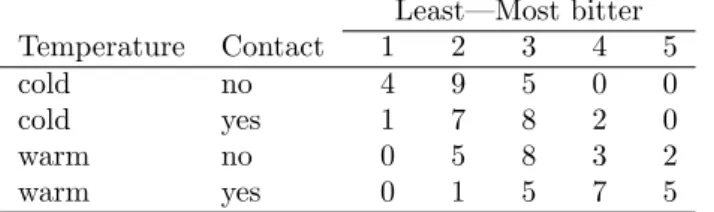
Table 1: Wine data from Randall (1989). Least—Most bitter Temperature Contact 1 2 3 4 5 cold no 4 9 5 0 0 cold yes 1 7 8 2 0 warm no 0 5 8 3 2 warm yes 0 1 5 7 5

consider the wine data from Randall (1989) available in the objectwinein packageordinal_{, cf.}

Table 1. The data represent a factorial experiment on factors determining the bitterness of wine with 1 = “least bitter” and 5 = “most bitter”. Two treatment factors (temperature and contact) each have two levels. Temperature and contact between juice and skins can be controlled when crushing grapes during wine production. Nine judges each assessed wine from two bottles from each of the four treatment conditions, hence there are 72 observations in all. In Table 1 we have aggregated data over bottles and judges for simplicity, but these variables will be considered later. Initially we only assume that, say, category 4 is larger than 3, but not that the distance between 2 and 3 is half the distance between 2 and 4, for example. The main objective is to examine the effect of contact and temperature on the perceived bitterness of wine.

2 Cumulative link models

A cumulative link model is a model for an ordinal response variable, Yi that can fall in j = 1, . . . , J categories.1 _Then _Yi _{follows a multinomial distribution with parameter} _π

where πij denote the probability that the ith observation falls in response category j. We define the cumulative probabilities as2

γij =P(Yi≤j) =πi1+. . .+πij . (1)

Initially we will consider the logit link. The logit function is defined as logit(π) = log[π/(1− π)] and cumulative logits are defined as:

logit(γij) = logit(P(Yi≤j)) = log P(Yi≤j)

1−P(Yi≤j) j= 1, . . . , J−1 (2) so that the cumulative logits are defined for all but the last category.3

A cumulative link model with a logit link, or simplycumulative logit model is a regression model for cumulative logits:

logit(γij) =θj−xT_iβ (3)

wherexiis a vector of explanatory variables for theith observation andβis the correspond-ing set of regression parameters. The {θj} parameters provide each cumulative logit (for eachj) with its own intercept. A key point is that the regression partxT_i βis independent ofj, soβ has the same effect for each of the J−1 cumulative logits. Note thatxT_i βdoes

1

whereJ ≥2. IfJ = 2 binomial models also apply, and in fact the cumulative link model is in this situation identical to a generalized linear model for a binomial response.

2

we have suppressed the conditioning on the covariate vector,xi, so we have thatγij = γj(xi) and

P(Yi≤j) =P(Y ≤j|xi).

3

(5)

0 1 x_iTβ γij = P ( Yi ≤ j ) j=1 j=2 j=3

Figure 1: Illustration of a cumulative link model with four response categories. Table 2: Estimates from ordinary logistic regression models (OLR) and a cumulative logit model (CLM) fitted to the wine data (cf. Table 1).

OLR CLM

j Intercept contact θj contact

1 -2.08 -1.48(1.14) -2.14 1.21(0.45)

2 0.00 -1.10(0.51) 0.04

3 1.82 -1.37(0.59) 1.71

4 2.83 -1.01(0.87) 2.98

not contain an intercept, since the {θj} act as intercepts. The cumulative logit model is illustrated in Fig. 1 for data with four response categories. For small values of xT

i β the response is likely to fall in the first category and for large values of xT_i β the response is likely to fall in the last category. The horizontal displacements of the curves are given by the values of{θj}.

Some sources write the cumulative logit model, (3) with a plus on the right-hand-side, but there are two good reasons for the minus. First, it means that the larger the value ofxT

i β, the higher the probability of the response falling in a category at the upper end of the response scale. Thus β has the same direction of effect as the regression parameter in an ordinary linear regression or ANOVA model. The second reason is related to the latent variable interpretation of cumulative link models that we will consider in section 2.6.

Example 2: We will consider a cumulative logit model for the wine data including an effect of contact. The response variable is the bitterness ratings, thus eachyi takes a value from 1 to 5 representing the degree of bitterness for theith sample. We may write the cumulative logit model as:

logit(γij) =θj−β2(contact_i), j= 1, . . . ,4, i= 1, . . . ,72.

The parameter estimates are given in the last two columns of Table 2. If we consider the cumulative logit model (3) for a fixed j, e.g., for j = 1, then the model is just a ordinary logistic regression model where the binomial response is divided into those observations falling in category j or less (Yi ≤ j), and those falling in a higher category than j (Yi > j). An initial analysis might indeed start by fitting such an ordinary logistic regression models for a dichotomized response. If we proceed in this vein, we could fit theJ−1 = 4 ordinary logistic

(6)

regression model by fixing j at 1, 2, 3, and 4 in turn. The estimates of those four ordinary logistic regression models are given in Table 2 under the OLR heading. The cumulative logit model can be seen as the model that combines these four ordinary logistic regression models into a single model and therefore makes better use of the information in the data. A part from a sign difference the estimate of the effect of contactfrom the cumulative logit model is about the average of thecontact effect estimates from the ordinary logistic regression models. Also observe that the standard error of the contacteffect is smaller in the cumulative logit model than in any of the ordinary logistic regression models reflecting that the effect ofcontactis more accurately determined in the cumulative logit model. The intercepts from the ordinary logistic regression models are also seen to correspond to the threshold parameters in the cumulative logit model.

The four ordinary logistic regression models can be combined in a single ordinary logistic re-gression model providing an even better approximation to the cumulative link model. This is

considered further in Appendix A.

2.1 Fitting cumulative link models with

clm

_{from package}

ordinal

Cumulative link models can be fitted withclmfrom packageordinal_{. The function takes the}

following arguments:

function (formula, scale, nominal, data, weights, start, subset, doFit = TRUE, na.action, contrasts, model = TRUE, control = list(), link = c("logit",

"probit", "cloglog", "loglog", "cauchit"), threshold = c("flexible", "symmetric", "symmetric2", "equidistant"), ...)

Most arguments are standard and well-known fromlm andglm, so they will not be intro-duced. The formula argument is of the form response ~ covariates and specifies the linear predictor. Theresponseshould be anordered factor (seehelp(factor)) with levels corresponding to the response categories. A number of link functions are available and the logit link is the default. The doFit and threshold arguments will be introduced in later sections. For further information about the arguments see the help page forclm4_.

Example 3: In this example we fit a cumulative logit model to the wine data presented in example 1 with clm from package ordinal_{. A cumulative logit model that includes additive}

effects of temperature and contact is fitted and summarized with > fm1 <- clm(rating ~ contact + temp, data = wine) > summary(fm1)

formula: rating ~ contact + temp

data: wine

link threshold nobs logLik AIC niter max.grad cond.H logit flexible 72 -86.49 184.98 6(0) 4.01e-12 2.7e+01 Coefficients:

Estimate Std. Error z value Pr(>|z|)

contactyes 1.5278 0.4766 3.205 0.00135 **

tempwarm 2.5031 0.5287 4.735 2.19e-06 ***

---Signif. codes: 0 ‘***’ 0.001 ‘**’ 0.01 ‘*’ 0.05 ‘.’ 0.1 ‘ ’ 1

4

(7)

Threshold coefficients:

Estimate Std. Error z value

1|2 -1.3444 0.5171 -2.600

2|3 1.2508 0.4379 2.857

3|4 3.4669 0.5978 5.800

4|5 5.0064 0.7309 6.850

The summary provides basic information about the model fit. There are two coefficient tables: one for the regression variables and one for the thresholds or cut-points. Often the thresholds are not of primary interest, but they are an integral part of the model. It is not relevant to test whether the thresholds are equal to zero, so nop-values are provided for this test. The condition number of the Hessian is a measure of how identifiable the model is; large values, say larger than1e4indicate that the model may be ill defined. From this model it appears that contact and high temperature both lead to higher probabilities of observations in the high categories as we would also expect from examining Table 1.

The Wald tests provided by summary indicate that both contact and temperature effects are strong. More accurate likelihood ratio tests can be obtained using thedrop1andadd1methods (equivalentlydroptermoraddterm). The Wald tests are marginal tests so the test of e.g.,temp

is measuring the effect of temperature whilecontrolling for the effect of contact. The equivalent likelihood ratio tests are provided by thedrop-methods:

> drop1(fm1, test = "Chi")

Single term deletions Model:

rating ~ contact + temp

Df AIC LRT Pr(>Chi) <none> 184.98 contact 1 194.03 11.043 0.0008902 *** temp 1 209.91 26.928 2.112e-07 *** ---Signif. codes: 0 ‘***’ 0.001 ‘**’ 0.01 ‘*’ 0.05 ‘.’ 0.1 ‘ ’ 1

In this case the likelihood ratio tests are slightly more significant than the Wald tests. We could also have tested the effect of the variables while ignoringthe effect of the other variable. For this test we use theadd-methods:

> fm0 <- clm(rating ~ 1, data = wine)

> add1(fm0, scope = ~ contact + temp, test = "Chi")

Single term additions Model: rating ~ 1 Df AIC LRT Pr(>Chi) <none> 215.44 contact 1 209.91 7.5263 0.00608 ** temp 1 194.03 23.4113 1.308e-06 *** ---Signif. codes: 0 ‘***’ 0.001 ‘**’ 0.01 ‘*’ 0.05 ‘.’ 0.1 ‘ ’ 1

where we used the scopeargument to indicate which terms to include in the model formula. These tests are a little less significant than the tests controlling for the effect of the other variable. Conventional symmetric so-called Wald confidence intervals for the parameters are available as > confint(fm1, type = "Wald")

(8)

2.5 % 97.5 % 1|2 -2.3578848 -0.330882 2|3 0.3925794 2.109038 3|4 2.2952980 4.638476 4|5 3.5738541 6.438954 contactyes 0.5936345 2.461961 tempwarm 1.4669081 3.539296

More accurate profile likelihood confidence intervals are also available and these are discussed

in section 4.

2.2 Odds ratios and proportional odds

The odds ratio of the eventY ≤j atx1relative to the same event atx2 is

OR = γj(x1)/[1−γj(x1)] γj(x2)/[1−γj(x2)] = exp(θj−x T 1β) exp(θj−xT₂β)= exp[(x T 2 −xT1)β]

which is independent of j. Thus the cumulative odds ratio is proportional to the distance between x1 and x2 which made McCullagh (1980) call the cumulative logit model a

pro-portional odds model. Ifxrepresent a treatment variable with two levels (e.g., placebo and treatment), thenx2−x1= 1 and the odds ratio is exp(−βtreatment). Similarly the odds ratio

of the eventY ≥j is exp(βtreatment).

Confidence intervals for the odds ratios are obtained by transforming the limits of confi-dence intervals forβ, which will lead to asymmetric confidence intervals for the odds ratios. Symmetric confidence intervals constructed from the standard error of the odds ratios will not be appropriate and should be avoided.

Example 4: The (cumulative) odds ratio ofrating≥j(for allj= 1, . . . , J−1) for contact and temperature are

> round(exp(fm1$beta), 1)

contactyes tempwarm

4.6 12.2

attesting to the strong effects of contact and temperature. Asymmetric confidence intervals for the odds ratios based on the Wald statistic are:

> round(exp(confint(fm1, type = "Wald")), 1)

2.5 % 97.5 % 1|2 0.1 0.7 2|3 1.5 8.2 3|4 9.9 103.4 4|5 35.7 625.8 contactyes 1.8 11.7 tempwarm 4.3 34.4

(9)

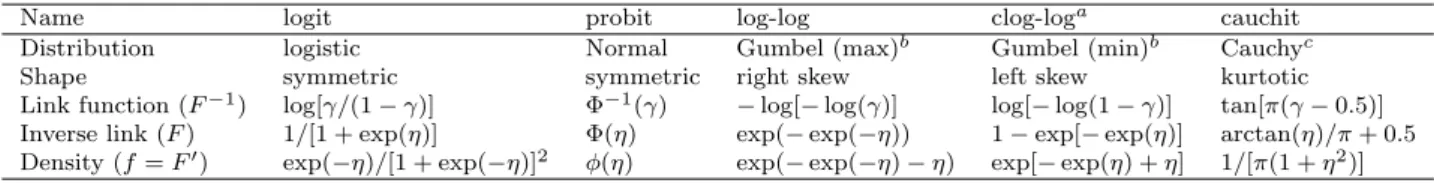
Table 3: Summary of various link functions

Name logit probit log-log clog-loga _cauchit

Distribution logistic Normal Gumbel (max)b _{Gumbel (min)}b _Cauchyc

Shape symmetric symmetric right skew left skew kurtotic

Link function (F−1

) log[γ/(1−γ)] Φ−1

(γ) −log[−log(γ)] log[−log(1−γ)] tan[π(γ−0.5)] Inverse link (F) 1/[1 + exp(η)] Φ(η) exp(−exp(−η)) 1−exp[−exp(η)] arctan(η)/π+ 0.5 Density (f=F′₎ _exp(−_η₎_/_{[1 + exp(−}_η_)]2

φ(η) exp(−exp(−η)−η) exp[−exp(η) +η] 1/[π(1 +η2

)]

a_{: the}_{complementary log-log}_link

b_: _{the Gumbel distribution is also known as the extreme value (type I) distribution for extreme}

minima or maxima. It is also sometimes referred to as the Weibull (or log-Weibull) distribution (http://en.wikipedia.org/wiki/Gumbel_distribution).

c_{: the Cauchy distribution is a}_t_{-distribution with one df}

2.3 Link functions

Cumulative link models are not formally a member of the class of (univariate) generalized linear models5_{(McCullagh and Nelder, 1989), but they share many similarities with}

gener-alized linear models. Notably a link function and a linear predictor (ηij =θj−xT_iβ) needs to be specified as in generalized linear models while the response distribution is just the multinomial. Fahrmeir and Tutz (2001) argues that cumulative link models are members of a class of multivariate generalized linear models. In addition to the logit link other choices are the probit, cauchit, log-log and clog-log links. These are summarized in Table 3. The cumulative link model may be written as

γij =F(ηij), ηij =θj−xTiβ (4) whereF−1 _{is the link function—the motivation for this particular notation will be given in}

section 2.6.

The probit link is often used when the model is interpreted with reference to a latent variable, cf. section 2.6. When the response variable represent grouped duration or survival times the complementary log-log link is often used. This leads to the proportional hazard model for grouped responses:

−log{1−γj(xi)}= exp(θj−xTiβ) or equivalently

log[−log{1−γj(xi)}] =θj−xT_iβ . (5) Here 1−γj(xi) is the probability or survival beyond categoryj givenxi. The proportional hazards model has the property that

log{γj(x1)}= exp[(xT2 −xT1)β] log{γj(x2)}.

If the log-log link is used on the response categories in the reverse order, this is equivalent to using the c-log-log link on the response in the original order. This reverses the sign of β as well as the sign and order of {θj} while the likelihood and standard errors remain unchanged.

5

the distribution of the response, the multinomial, is not a member of the (univariate) exponential family of distributions.

(10)

Table 4: Income distribution (percentages) in the Northeast US adopted from McCullagh (1980). Year Income 0-3 3-5 5-7 7-10 10-12 12-15 15+ 1960 6.50 8.20 11.30 23.50 15.60 12.70 22.20 1970 4.30 6.00 7.70 13.20 10.50 16.30 42.10

In addition to the standard links in Table 3, flexible link functions are available forclmin packageordinal_.

Example 5: McCullagh (1980) present data on income distribution in the Northeast US repro-duced in Table 4 and available in packageordinal_{as the object}_income_{. The unit of the income}

groups are thousands of (constant) 1973 US dollars. The numbers in the body of the table are percentages of the population summing to 100 in each row6

, so these are not the original obser-vations. The uncertainty of parameter estimates depends on the sample size, which is unknown here, so we will not consider hypothesis tests. Rather the most important systematic component is an upward shift in the income distribution from 1960 to 1970 which can be estimated from a cumulative link model. This is possible since the parameter estimates themselves only depend on the relative proportions and not the absolute numbers.

McCullagh considers which of the logit or cloglog links best fit the data in a model with an additive effect of year. He concludes that a the complementary log-log link corresponding to a right-skew distribution is a good choice. We can compare the relative merit of the links by comparing the value of the log-likelihood of models with different link functions:

> links <- c("logit", "probit", "cloglog", "loglog", "cauchit") > sapply(links, function(link) {

clm(income ~ year, data=income, weights=pct, link=link)$logLik })

logit probit cloglog loglog cauchit

-353.3589 -353.8036 -352.8980 -355.6028 -352.8434

The cauchit link attains the highest log-likelihood closely followed by the complementary log-log link. This indicates that a symmetric heavy tailed distribution such as the Cauchy provides an even slightly better description of these data than a right skew distribution.

Adopting the complementary log-log link we can summarize the connection between the income in the two years by the following: If p1960(x) is proportion of the population with an income

larger than $xin 1960 andp1970(x) is the equivalent in 1970, then approximately

logp1960(x) = exp( ˆβ) logp1970(x)

= exp(0.568) logp1970(x)

2.4 Maximum likelihood estimation of cumulative link models

Cumulative link models are usually estimated by maximum likelihood (ML) and this is also the criterion used in package ordinal_{. The log-likelihood function (ignoring additive}

constants) can be written as

ℓ(θ,β;y) = n X i=1 wilogπi (6) 6

(11)

whereiindex all scalar observations (not multinomial vector observations),wi are potential case weights andπi is the probability of theith observation falling in the response category that it did, i.e.,πiare the non-zero elements ofπijI(Yi =j). Here I(·) is the indicator function being 1 if its argument is true and zero otherwise. The ML estimates of the parameters; ˆθ and ˆβare those values of θ andβthat maximize the log-likelihood function in (6).

Not all data sets can be summarized in a table like Table 1. If a continuous variable takes a unique value for each observation, each row of the resulting table would contain a single 1 and zeroes for the rest. In this case all{wi}are one unless the observations are weighted for some other reason. If the data can be summarized as in Table 1, a multinomial observation vector such as [3,1,2] can be fitted usingy = [1,1,1,2,3,3] with w = [1,1,1,1,1,1] or by using y= [1,2,3] withw= [3,1,2]. The latter construction is considerably more computationally efficient (an therefore faster) since the log-likelihood function contains three rather than six terms and the design matrix,X will have three rather than six rows.

The details of the actual algorithm by which the likelihood function is optimized is deferred to a later section.

According to standard likelihood theory, the variance-covariance matrix of the parameters can be obtained as the inverse of the observed Fisher information matrix. This matrix is given by the negative Hessian of the log-likelihood function7 _{evaluated at the maximum}

likelihood estimates. Standard errors can be obtained as the square root of the diagonal of the variance-covariance matrix.

Letα = [θ,β] denote the full set of parameters. The Hessian matrix is then given as the second order derivative of the log-likelihood function evaluated at the ML estimates:

H= ∂ 2_ℓ₍_α_;_y₎ ∂α∂αT _α = ˆα . (7)

The observed Fisher information matrix is then I( ˆα) = −H and the standard errors are given by

se( ˆα) =pdiag[I( ˆα)−1_{] =}p_diag[₋_H_{( ˆ}_α₎−1_]_. ₍₈₎

Another general way to obtain the variance-covariance matrix of the parameters is to use the expected Fisher information matrix. The choice of whether to use the observed or the expected Fisher information matrix is often dictated by the fitting algorithm: re-weighted least squares methods often produce the expected Fisher information matrix as a by-product of the algorithm, and Newton-Raphson algorithms (such as the one used forclminordinal₎

similarly produce the observed Fisher information matrix. Efron and Hinkley (1978) consid-ered the choice of observed versus expected Fisher information and argued that the observed information contains relevant information thus it is preferred over the expected information. Pratt (1981) and Burridge (1981) showed (seemingly independent of each other) that the log-likelihood function of cumulative link models with the link functions considered in Table 3, except for the cauchit link, is concave. This means that there is a unique global optimum so there is no risk of convergence to a local optimum. It also means that the step of a Newton-Raphson algorithm is guarantied to be in the direction of a higher likelihood although the step may be too larger to cause an increase in the likelihood. Successively halving the step whenever this happens effectively ensures convergence.

7

(12)

Notably the log likelihood of cumulative cauchit models is not guarantied to be concave, so convergence problems may occur with the Newton-Raphson algorithm. Using the estimates from a cumulative probit models as starting values seems to be a widely successful approach. Observe also that the concavity property does not extend to cumulative link models with scale effects, but that structured thresholds (cf. section 2.7) are included.

2.5 Deviance and model comparison

2.5.1 Model comparison with likelihood ratio tests

A general way to compare models is by means of the likelihood ratio statistic. Consider two models, m0 andm1, wherem0 is a submodel of model m1, that is, m0 is simpler thanm1

andm0 isnested in m1. The likelihood ratio statistic for the comparison of m0andm1is

LR=−2(ℓ0−ℓ1) (9)

whereℓ0 is the log-likelihood of m0 andℓ1 is the log-likelihood ofm1. The likelihood ratio

statistic measures the evidence in the data for the extra complexity in m1 relative to m0.

The likelihood ratio statistic asymptotically follows aχ2_{distribution with degrees of freedom}

equal to the difference in the number of parameter ofm0andm1. The likelihood ratio test

is generally more accurate than Wald tests. Cumulative link models can be compared by means of likelihood ratio tests with theanovamethod.

Example 6: Consider the additive model for the wine data in example 3 with a main effect of temperature and contact. We can use the likelihood ratio test to assess whether the interaction between these factors are supported by the data:

> fm2 <- clm(rating ~ contact * temp, data = wine) > anova(fm1, fm2)

Likelihood ratio tests of cumulative link models:

formula: link: threshold:

fm1 rating ~ contact + temp logit flexible fm2 rating ~ contact * temp logit flexible

no.par AIC logLik LR.stat df Pr(>Chisq)

fm1 6 184.98 -86.492

fm2 7 186.83 -86.416 0.1514 1 0.6972

The likelihood ratio statistic is small in this case and compared to aχ2

distribution with 1 df, the p-value turns out insignificant. We conclude that the interaction is not supported by the

data.

2.5.2 Deviance and ANODE tables

In linear models ANOVA tables and F-tests are based on the decomposition of sums of squares. The concept of sums of squares does not make much sense for categorical observa-tions, but a more general measure called thedevianceis defined for generalized linear models and contingency tables8_{. The deviance can be used in much the same way to compare nested}

8

(13)

models and to make a so-called analysis of deviance (ANODE) table. The deviance is closely related to sums of squares for linear models (McCullagh and Nelder, 1989).

The deviance is defined as minus twice the difference between the log-likelihoods of a full (orsaturated) model and a reduced model:

D=−2(ℓreduced−ℓfull) (10)

The full model has a parameter for each observation and describes the data perfectly while the reduced model provides a more concise description of the data with fewer parameters. A special reduced model is thenull model which describes no other structure in the data than what is implied by the design. The corresponding deviance is known as thenull deviance and analogous to the total sums of squares for linear models. The null deviance is therefore also denoted the total deviance. The residual deviance is a concept similar to a residual sums of squares and simply defined as

Dresid=Dtotal−Dreduced (11)

Adifference in deviancebetween two nested models is identical to the likelihood ratio statis-tic for the comparison of these models. Thus the deviance difference, just like the likelihood ratio statistic, asymptotically follows aχ2_{-distribution with degrees of freedom equal to the}

difference in the number of parameters in the two models. In fact the deviance in (10) is just the likelihood ratio statistic for the comparison of the full and reduced models. The likelihood of reduced models are available from fits of cumulative link models, but since it is not always easy to express the full model as a cumulative link model, the log-likelihood of the full model has to be obtained in another way. For a two-way table like Table 1 indexed byh(rows) andj(columns), the log-likelihood of the full model (comparable to the likelihood in (6)) is given by ℓfull= X h X j whjlog ˆπhj (12)

where ˆπhj=whj/wh.,whj is the count in the (h, j)th cell and wh. is the sum in rowh.

Example 7: We can get the likelihood of the full model for the wine data in Table 1 with > tab <- with(wine, table(temp:contact, rating))

> ## Get full log-likelihood: > pi.hat <- tab / rowSums(tab)

> (ll.full <- sum(tab * ifelse(pi.hat > 0, log(pi.hat), 0))) ## -84.01558

[1] -84.01558

The total deviance (10) for the wine data is given by > ## fit null-model:

> fm0 <- clm(rating ~ 1, data = wine) > ll.null <- fm0$logLik

> ## The null or total deviance:

> (Deviance <- -2 * (ll.null - ll.full)) ## 39.407

[1] 39.407

Example 8: An ANODE table for the wine data in Table 1 is presented in Table 5 where the total deviance is broken up into model deviance (due to treatments) and residual deviance.

(14)

Table 5: ANODE table for the data in Table 1.

Source df deviance p-value

Total 12 39.407 <0.001 Treatment 3 34.606 <0.001 Temperature,T 1 26.928 <0.001 Contact,C 1 11.043 <0.001 Interaction,T×C 1 0.1514 0.6972 Residual 9 4.8012 0.8513

Further, the treatment deviance is described by contributions from main effects and interaction. Observe that the deviances for the main effects and interaction do not add up to the deviance for Treatment as the corresponding sums of squares would have in a analogous linear model (ANOVA)9

. The deviances for these terms can instead be interpreted as likelihood ratio tests of nested models: the deviance for the interaction term is the likelihood ratio statistics of the interaction controlling for the main effects, and the deviances for the main effects are the likelihood ratio statistics for these terms while controlling for the other main effect and ignoring the interaction term. As is clear from Table 5, there are significant treatment differences and these seem to describe the data well since the residual deviance is insignificant—the latter is a goodness of fit test for the cumulative logit model describing treatment differences. Further, the treatment differences are well captured by the main effects and there is no indication of an

important interaction.

The terminology can be a bit confusing in this area. Sometimes any difference in deviance between two nested models, i.e., a likelihood ratio statistic is denoted a deviance and some-times any quantity that is proportional to minus twice the log-likelihood of a model is denoted the deviance of that model.

2.5.3 Goodness of fit tests with the deviance

The deviance can be used to test the goodness of fit of a particular reduced model. The deviance asymptotically follows asχ2 _{distribution with degrees of freedom equal to the}

dif-ference in the number of parameters between the two models. The asymptotics are generally good if the expected frequencies under the reduced model are not too small and as a general rule they should all be at least five. This provides a goodness of fit test of the reduced model. The expectation of a random variable that follows aχ2_{-distribution is equal to the}

degrees of freedom of the distribution, so as a rule of thumb, if the deviance in (10) is about the same size as the difference in the number of parameters, there is not evidence of lack of fit.

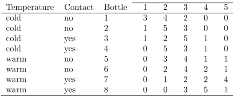
One problem with the deviance for a particular (reduced) model is that it depends on which model is considered the full model, i.e., how the total deviance is calculated, which often derives from the tabulation of the data. Observe that differences in deviance for nested models are independent of the likelihood of a full model, so deviance differences are insensitive to this choice. Collett (2002) recommends that the data are aggregated as much as possible when evaluating deviances and goodness of fit tests are performed.

Example 9: In the presentation of the wine data in example 1 and Table 1, the data were aggregated over judges and bottles. Had we includedbottle in the tabulation of the data we

9

(15)

Table 6: Table of the wine data similar to Table 1, but including bottle in the tabulation. Least—Most bitter

Temperature Contact Bottle 1 2 3 4 5

cold no 1 3 4 2 0 0 cold no 2 1 5 3 0 0 cold yes 3 1 2 5 1 0 cold yes 4 0 5 3 1 0 warm no 5 0 3 4 1 1 warm no 6 0 2 4 2 1 warm yes 7 0 1 2 2 4 warm yes 8 0 0 3 5 1

would have arrived at Table 6. A full model for the data in Table 1 has (5−1)(4−1) = 12 degrees of freedom while a full model for Table 6 has (5−1)(8−1) = 28 degrees of freedom and a different deviance.

If it is decided that bottle is not an important variable, Collett’s recommendation is that we base the residual deviance on a full model defined from Table 1 rather than Table 6.

2.6 Latent variable motivation for cumulative link models

A cumulative link model can be motivated by assuming an underlying continuous latent variable, S with cumulative distribution function, F. The ordinal response variable, Yi is then observed in categoryj ifSi is between the thresholdsθ∗

j−1< Si≤θj∗where −∞ ≡θ∗

0 < θ∗1< . . . < θJ∗−1< θ∗J≡ ∞

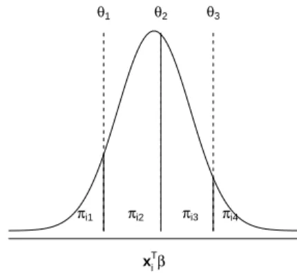
divide the real line on whichSlives intoJ+ 1 intervals. The situation is illustrated in Fig. 2 where a probit link and J = 4 is adopted. The three thresholds, θ1, θ2, θ3 divide the area

under the curve into four parts each of which represent the probability of a response falling in the four response categories. The thresholds are fixed on the scale, but the location of the latent distribution, and therefore also the four areas under the curve, changes withxi. A normal linear model for the latent variable is

Si=α+xTi β∗+εi , εi∼N(0, σ2) (13) where{εi}are random disturbances andαis the intercept, i.e., the mean value ofSiwhenxi correspond to a reference level for factors and to zero for continuous covariates. Equivalently we could write: Si∼N(α+xTiβ∗, σ2).

The cumulative probability of an observation falling in categoryj or below is then: γij=P(Yi≤j) =P(Si≤θ∗ j) =P Zi≤ θ∗ j −α−xTiβ∗ σ ! = Φ θ ∗ j−α−xTi β∗ σ ! (14) whereZi= (Si−α−xT

iβ∗)/σ∼N(0,1) and Φ is the standard normal CDF.

Since the absolute location and scale of the latent variable, α and σ respectively, are not identifiable from ordinal observations, an identifiable model is

(16)

θ1 θ2 θ3

πi1 πi2 πi3 πi4

x_iTβ

Figure 2: Illustration of a cumulative link model in terms of the latent distribution. with identifiable parameter functions:

θj = (θ∗

j −α)/σ and β=β∗/σ . (16) Observe how the minus in (15) entered naturally such that a positiveβ means a shift of the latent distribution in a positive direction.

Model (15) is exactly a cumulative link model with a probit link. Other distributional as-sumptions forS correspond to other link functions. In general assuming that the cumulative distribution function ofSisF corresponds to assuming the link function isF−1_{, cf. Table 3.}

Some expositions of the latent variable motivation for cumulative link models get around the identifiability problem by introducing restrictions onαandσ, usuallyα= 0 andσ= 1 are chosen, which leads to the same definition of the threshold and regression parameters that we use here. However, it seems misleading to introduce restrictions on unidentifiable parameters. If observations really arise from a continuous latent variable,αand σare real unknown parameters and it makes little sense to restrict them to take certain values. This draws focus from the appropriate relative signal-to-ratio interpretation of the parameters evident from (16).

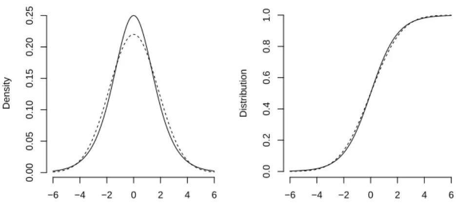
The standard form of the logistic distribution has mean zero and varianceπ2_/_{3. The logistic}

distribution is symmetric and shows a some resemblance with a normal distribution with the same mean and variance in the central part of the distribution; the tails of the logistic distribution are a little heavier than the tails of the normal distribution. In Fig. 3 the normal and logistic distributions are compared with variance π2_/_{3. Therefore, to a reasonable}

approximation, the parameters of logit and probit models are related in the following way: θprobit_j ≈θlogit_j /(π/√3) and βprobit≈βlogit/(π/√3), (17) whereπ/√3≈1.81

Example 10: Considering once again the wine data the coefficients from logit and probit mod-els with additive effects of temperature and contact are

> fm1 <- clm(rating ~ contact + temp, data = wine, link = "logit") > fm2 <- clm(rating ~ contact + temp, data = wine, link = "probit") > structure(rbind(coef(fm1), coef(fm2)),

(17)

Density −6 −4 −2 0 2 4 6 0.00 0.05 0.10 0.15 0.20 0.25 Distr ib ution −6 −4 −2 0 2 4 6 0.0 0.2 0.4 0.6 0.8 1.0

Figure 3: Left: densities. Right: distributions of logistic (solid) and normal (dashed) distri-butions with mean zero and varianceπ2_/_{3 which corresponds to the standard form for the}

logistic distribution.

1|2 2|3 3|4 4|5 contactyes tempwarm

logit -1.3443834 1.2508088 3.466887 5.006404 1.5277977 2.503102 probit -0.7732627 0.7360215 2.044680 2.941345 0.8677435 1.499375

In comparison the approximate probit estimates using (17) are > coef(fm1) / (pi / sqrt(3))

1|2 2|3 3|4 4|5 contactyes tempwarm

-0.7411974 0.6896070 1.9113949 2.7601753 0.8423190 1.3800325

These estimates are a great deal closer to the real probit estimates than the unscaled logit estimates. The average difference between the probit and approximate probit estimates being

-0.079.

2.6.1 More on parameter interpretation

Observe that the regression parameter in cumulative link models, cf. (16) are signal-to-noise ratios. This means that adding a covariate to a cumulative link model that reduces the residual noise in the corresponding latent model will increase the signal-to-noise ratios. Thus adding a covariate will (often) increase the coefficients of the other covariates in the cumulative link model. This is different from linear models, where (in orthogonal designs) adding a covariate does not alter the value of the other coefficients10_{. Bauer (2009),}

extend-ing work by Winship and Mare (1984) suggests a way to rescale the coefficients such they are comparable in size during model development. See also Fielding (2004).

Example 11: Consider the estimate oftempin models for the wine data ignoring and control-ling forcontact, respectively:

> coef(clm(rating ~ temp, data = wine, link = "probit"))["tempwarm"]

tempwarm 1.37229

10

but the same thing happens in other generalized linear models, e.g., binomial and Poisson models, where the variance is determined by the mean.

(18)

> coef(clm(rating ~ temp + contact, data = wine, link = "probit"))["tempwarm"]

tempwarm 1.499375

and observe that the estimate of temp is larger when controlling forcontact. In comparison the equivalent estimates in linear models are not affected—here we use the observed scores for illustration:

> coef(lm(as.numeric(rating) ~ temp, data = wine))["tempwarm"]

tempwarm 1.166667

> coef(lm(as.numeric(rating) ~ contact + temp, data = wine))["tempwarm"]

tempwarm 1.166667

In this case the coefficients are exactly identical, but in designs that are not orthogonal and observed studies with correlated covariates they will only be approximately the same.

Regardless of how the threshold parameters discretize the scale of the latent variable, the regression parameters β have the same interpretation. Thus β have the same meaning whether the ordinal variable is measured in, say, five or six categories. Further, the nature of the model interpretation will not chance if two or more categories are amalgamated, while parameter estimates will, of course, not be completely identical. This means that regression parameter estimates can be compared (to the extent that the noise level is the same) across studies where response scales with a different number of response categories are adopted. In comparison, for linear models used on scores, it is not so simple to just combine two scores, and parameter estimates from different linear models are not directly comparable.

If the latent variable,Si is approximated by scores assigned to the response variable, denote this variable Y∗

i , then a linear model for Yi∗ can provide approximate estimates of β by applying (16) for cumulative probit models11_{. The quality of the estimates rest on a number}

of aspects:

• The scores assigned to the ordinal response variable should be structurally equivalent to the thresholds, θ∗ _{that generate} _Yi _from _Si_{. In particular, if the (equidistant)}

numbers 1, . . . , J are the scores assigned to the response categories, the thresholds,θ∗

are also assumed to be equidistant. • The distribution ofY∗

i should not deviate too much from a bell-shaped curve; especially there should not be too many observations in the end categories

• By appeal to the central limit theorem the coarsening ofSiintoY∗

i will “average out” such that bias due to coarsening is probably small.

This approximate estimation scheme extends to other latent variable distributions than the normal where linear models are exchanged with the appropriate location-scale models, cf. Table 3.

11

these approximate regression parameters could be used as starting values for an iterative algorithm to find the ML estimates ofβ, but we have not found it worth the trouble in our Newton algorithm

(19)

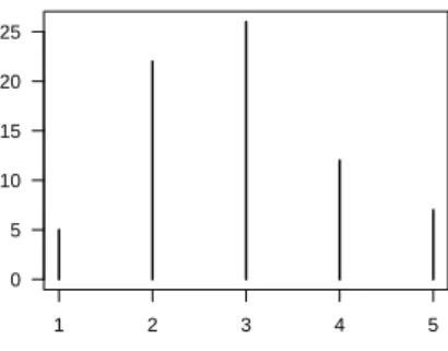
0 5 10 15 20 25 1 2 3 4 5

Figure 4: Histogram of the ratings in the wine data, cf. Table 1.

Example 12: Consider the following linear model for the rating scores of the wine data, cf. Table 1:

Y∗

i =α+β1temp_i+β2contacti+εi εi ∼N(0, σ

2

ε) The relative parameter estimates, ˜βare

> lm1 <- lm(as.numeric(rating) ~ contact + temp, data =wine) > sd.lm1 <- summary(lm1)$sigma

> coef(lm1)[-1] / sd.lm1

contactyes tempwarm 0.791107 1.384437

which should be compared with the estimates from the corresponding cumulative probit model: > fm1 <- clm(rating ~ contact + temp, data = wine, link = "probit")

> coef(fm1)[-(1:4)]

contactyes tempwarm 0.8677435 1.4993746

The relative estimates from the linear model are a lower than the cumulative probit estimates, which is a consequence of the fact that the assumptions for the linear model are not fulfilled. In particular the distance between the thresholds is not equidistant:

> diff(coef(fm1)[1:4])

2|3 3|4 4|5

1.5092842 1.3086590 0.8966645

while the distribution is probably sufficiently bell-shaped, cf. Fig 4.

2.7 Structured thresholds

In this section we will motivate and describe structures on the thresholds in cumulative link models. Three options are available in clmusing thethreshold argument: flexible, sym-metric and equidistant thresholds. The default option is "flexible", which corresponds to the conventional ordered, but otherwise unstructured thresholds. The"symmetric" op-tion restricts the thresholds to be symmetric while the"equidistant"option restricts the

(20)

Table 7: Symmetric thresholds with six response categories use the three parameters a, b andc.

θ1 θ2 θ3 θ4 θ5

−b+c −a+c c a+c b+c

Table 8: Symmetric thresholds with seven response categories use the four parameters,a,b, candd.

θ1 θ2 θ3 θ4 θ5 θ6

−b+c −a+c c d a+d b+d

thresholds to be equally spaced. 2.7.1 Symmetric thresholds

The basic cumulative link model assumed that the thresholds are constant for all values of xT_iβ, that they are ordered and finite but otherwise without structure. In questionnaire type response scales, the question is often of the form “how much do you agree with state-ment” with response categories ranging from “completely agree” to “completely disagree” in addition to a number of intermediate categories possibly with appropriate anchoring words. In this situation the response scale is meant to be perceived as being symmetric, thus, for example, the end categories are equally far from the central category/categories. Thus, in the analysis of such data it can be relevant to restrict the thresholds to be symmetric or at least test the hypothesis of symmetric thresholds against the more general alternative requiring only that the thresholds are ordered in the conventional cumulative link model. An example with six response categories and five thresholds is given in Table 7 where the central threshold,θ3 maps toc whileaand b arespacings determining the distance to the

remaining thresholds. Symmetric thresholds is a parsimonious alternative since three rather than five parameters are required to determine the thresholds in this case. Naturally at least four response categories, i.e., three thresholds are required for the symmetric thresholds to use less parameters than the general alternative. With an even number of thresholds, we use a parameterization with two central thresholds as shown in Table 8.

Example 13: I am missing some good data to use here.

2.7.2 Equidistant thresholds

Ordinal data sometimes arise when the intensity of some perception is rated on an ordinal response scale. An example of such a scale is the ratings of the bitterness of wine described in example 1. In such cases it is natural to hypothesize that the thresholds are equally spaced, or equidistant as we shall denote this structure. Equidistant thresholds use only two parameters and our parameterization can be described by the following mapping:

θj=a+b(j−1), for j= 1, . . . , J−1 (18) such thatθ1=ais the first threshold andbdenotes the distance between adjacent thresholds.

Example 14: In example 3 we fitted a model for the wine data (cf. Table 1) with additive effects of temperature and contact while only restricting the thresholds to be suitably ordered. For convenience this model fit is repeated here:

(21)

> fm1 <- clm(rating ~ temp + contact, data=wine) > summary(fm1)

formula: rating ~ temp + contact

data: wine

link threshold nobs logLik AIC niter max.grad cond.H logit flexible 72 -86.49 184.98 6(0) 4.01e-12 2.7e+01 Coefficients:

tempwarm 2.5031 0.5287 4.735 2.19e-06 ***

contactyes 1.5278 0.4766 3.205 0.00135 **

---Signif. codes: 0 ‘***’ 0.001 ‘**’ 0.01 ‘*’ 0.05 ‘.’ 0.1 ‘ ’ 1 Threshold coefficients:

1|2 -1.3444 0.5171 -2.600

2|3 1.2508 0.4379 2.857

3|4 3.4669 0.5978 5.800

4|5 5.0064 0.7309 6.850

The successive distances between the thresholds in this model are > diff(fm1$alpha)

2|3 3|4 4|5

2.595192 2.216078 1.539517

so the distance between the thresholds seems to be decreasing. However, the standard errors of the thresholds are about half the size of the distances, so their position is not that well determined. A model where the thresholds are restricted to be equally spaced is fitted with > fm2 <- clm(rating ~ temp + contact, data=wine, threshold="equidistant") > summary(fm2)

formula: rating ~ temp + contact

data: wine

link threshold nobs logLik AIC niter max.grad cond.H logit equidistant 72 -87.86 183.73 5(0) 4.80e-07 3.2e+01 Coefficients:

tempwarm 2.4632 0.5164 4.77 1.84e-06 ***

contactyes 1.5080 0.4712 3.20 0.00137 **

---Signif. codes: 0 ‘***’ 0.001 ‘**’ 0.01 ‘*’ 0.05 ‘.’ 0.1 ‘ ’ 1 Threshold coefficients:

threshold.1 -1.0010 0.3978 -2.517

spacing 2.1229 0.2455 8.646

so here ˆθ1 = ˆa = −1.001 and ˆb = 2.123 in the parameterization of (18). We can test the

(22)

> anova(fm1, fm2)

Likelihood ratio tests of cumulative link models:

formula: link: threshold:

fm2 rating ~ temp + contact logit equidistant fm1 rating ~ temp + contact logit flexible

no.par AIC logLik LR.stat df Pr(>Chisq)

fm2 4 183.73 -87.865

fm1 6 184.98 -86.492 2.7454 2 0.2534

so thep-value isp= 0.253 not providing much evidence against equidistant thresholds.

3 Assessing the likelihood and model convergence

Cumulative link models are non-linear models and in general the likelihood function of non-linear models is not guaranteed to be well behaved or even uni-modal. However, as mentioned in section 2.4 Pratt (1981) and Burridge (1981) showed that the log-likelihood function of cumulative link models with the link functions considered in Table 3, except for the cauchit link, is concave. This means that there is a unique global optimum so there is no risk of convergence to a local optimum. There is no such guarantee in more general models. There are no closed form expressions for the ML estimates of the parameters in cumulative link models. This means that iterative methods have to be used to fit the models. There is no guarantee that the iterative method converges to the optimum. In complicated models the iterative method may terminate at a local optimum or just far from the optimum resulting in inaccurate parameter estimates. We may hope that the optimization process warns about non-convergence, but that can also fail. To be sure the likelihood function is well behaved and that an unequivocal optimum has been reached we have to inspect the likelihood function in a neighborhood around the optimum as reported by the optimization.

As special feature for cumulative link models, the threshold parameters are restricted to be ordered and therefore naturally bounded. This may cause the log-likelihood function to be irregular for one or more parameters. This also motivates visualizing the likelihood function in the neighborhood of the optimum. To do this we use theslice function. As the name implies, it extracts a (one-dimensional) slice of the likelihood function.

We use the likelihood slices for two purposes:

1. To visualize and inspect the likelihood function in a neighborhood around the optimum. We choose a rather large neighborhood and look at how well-behaved the likelihood function is, how close to a quadratic function it is, and if there is only one optimum. 2. To verify that the optimization converged and that the parameter estimates are

ac-curately determined. For this we choose a rather narrow neighborhood around the optimum.

The log-likelihood slice is defined as

(23)

where α denotes the joint parameter vector. Thus the slice is the log-likelihood function regarded as a function of the ath parameter while the remaining parameters are fixed at their ML estimates.

The Hessian at the optimum measures the curvature in the log-likelihood function in the parameter space. To scale the range of the parameters at which the likelihood is sliced, we consider the following measures of curvature:

ζ=p

diag(−H) (20)

Here ζ is a (q+p)-vector of curvature units for the q threshold parameters θ and the p regression parameters β. We can understand ζ as a vector of standard errors which are not controlled for the dependency of the other parameters. Indeed, if the parameters are completely uncorrelated,His diagonal andζcoincide with standard errors, cf. (8), however, this is not possible in cumulative link models.

The range of the parameters at which the log-likelihood is sliced is then a simple multiple (λ) of the curvature units in each direction: λζ. Working in curvature units is a way to standardize the parameter range even if some parameters are much better determined (much less curvature in the log-likelihood) than others.

A well-behave log-likelihood function will be approximately quadratic in shape in a neigh-borhood around the optimum. Close enough to the optimum, the log-likelihood function will be virtually indistinguishable from a quadratic approximation if all parameters are iden-tified. For theath parameter the quadratic approximation to the log-likelihood function is given by −(ˆαa−αa) 2 2ζ2 a .

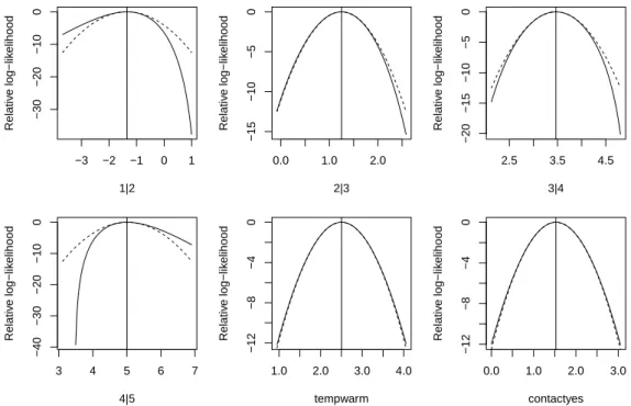
Example 15: Consider again a cumulative link model for the wine data. In the following we ask for a slice of the log-likelihood function for each of the parameters and plot these. By setting

λ= 5 we ask for the slice in a rather wide neighborhood around the optimum: > fm1 <- clm(rating ~ temp + contact, data=wine)

> slice.fm1 <- slice(fm1, lambda = 5) > par(mfrow = c(2, 3))

> plot(slice.fm1)

The result is shown in Fig. 5. By default the quadratic approximation is included for reference in the plot.

For this model we see that the log-likelihood function is nicely quadratic for the regression parameters while it is less so for the threshold parameters and particularly bad for the end thresholds. The log-likelihood isrelativeas indicated by the label on the vertical axis since the values are relative to the maximum log-likelihood value.

From Fig. 5 it seems that the parameter estimates as indicated by the vertical bars are close to the optimum indicating successful model convergence. To investigate more closely we slice the likelihood at a much smaller scale usingλ= 10−5

: > slice2.fm1 <- slice(fm1, lambda = 1e-5) > par(mfrow = c(2, 3))

> plot(slice2.fm1)

The resulting figure is shown in Fig. 6. Observe that 1) the model has converged, 2) from inspection of the horizontal axis all parameters estimates are correct to at least six decimals, 3) the quadratic approximation is indistinguishable from the log-likelihood at this scale and 4) from the vertical axis the log-likelihood value is determined accurately to at least 12 digits.

(24)

−3 −2 −1 0 1 −30 −20 −10 0 1|2 Relativ e log−lik elihood 0.0 1.0 2.0 −15 −10 −5 0 2|3 Relativ e log−lik elihood 2.5 3.5 4.5 −20 −15 −10 −5 0 3|4 Relativ e log−lik elihood 3 4 5 6 7 −40 −30 −20 −10 0 4|5 Relativ e log−lik elihood 1.0 2.0 3.0 4.0 −12 −8 −4 0 tempwarm Relativ e log−lik elihood 0.0 1.0 2.0 3.0 −12 −8 −4 0 contactyes Relativ e log−lik elihood

Figure 5: Slices of the log-likelihood function for parameters in a model for the bitterness-of-wine data. Dashed lines indicate quadratic approximations to the log-likelihood function and vertical bars indicate maximum likelihood estimates.

(25)

−1.344388−5e−11 −1.344382 −2e−11 0e+00 1|2 Relativ e log−lik elihood 1.250806−5e−11 1.250809 −2e−11 0e+00 2|3 Relativ e log−lik elihood 3.466885 3.466888 −5e−11 −2e−11 0e+00 3|4 Relativ e log−lik elihood 5.006402 5.006406 −5e−11 −2e−11 0e+00 4|5 Relativ e log−lik elihood 2.503099 2.503102 2.503105 −5e−11 −2e−11 0e+00 tempwarm Relativ e log−lik elihood 1.527795 1.527798 −5e−11 −2e−11 0e+00 contactyes Relativ e log−lik elihood

Figure 6: Slices of the log-likelihood function for parameters in a model for the bitterness-of-wine data very close to the MLEs. Dashed lines indicate quadratic approximations to the log-likelihood function and vertical bars the indicate maximum likelihood estimates.

Example 16: Example with confidence contours.

Unfortunately there is no general way to infer confidence intervals from the likelihood slices— for that we have to use the computationally more intensive profile likelihoods. Compared to the profile likelihoods discussed in section 4, the slice is much less computationally demand-ing since the likelihood function is only evaluated—not optimized, at a range of parameter values.

4 Confidence intervals and profile likelihood

Confidence intervals are convenient for summarizing the uncertainty about estimated pa-rameters. The classical symmetric estimates given by ˆβ ±z1−α/2se( ˆˆ β) are based on the

Wald statistic12_,_w₍_β_{) = ( ˆ}_β₋_β₎_/_{se( ˆ}_ˆ _β_{) and available by}_{confint(fm1, type = "Wald")}_{. A}

similar result could be obtained by confint.default(fm1). However, outside linear mod-els asymmetric confidence intervals often better reflect the uncertainty in the parameter estimates. More accurate, and generally asymmetric, confidence intervals can be obtained by using the likelihood root statistic instead; this relies on the so-called profile likelihood

12

(26)

written here for an arbitrary scalar parameterβa: ℓp(βa;y) = max

θ,β₋a

ℓ(θ,β;y),

whereβ₋a is the vector of regression parameters without theath one. In words, the profile log-likelihood forβa is given as the full log-likelihood optimized over all parameters butβa. To obtain a smooth function, the likelihood is optimized over a range of values ofβaaround the ML estimate, ˆβa, further, these points are interpolated by a spline to provide an even smoother function.

The likelihood root statistic (see e.g., Pawitan, 2001; Brazzale et al., 2007) is defined as: r(βa) = sign( ˆβa−βa)

q

−2[ℓ( ˆθ,βˆ;y)−ℓp(βa;y)]

and just like the Wald statistic its reference distribution is the standard normal. Confidence intervals based on the likelihood root statistic are defined as those values of βa for which r(βa) is in between specified bounds, e.g., −1.96 and 1.96 for 95% confidence intervals. Formally the confidence intervals are defined as

CI:

βa;|r(βa)|< z1−α/2 .

Example 17: Consider again a model for the wine data. The profile likelihood confidence intervals are obtained with

> fm1 <- clm(rating ~ temp + contact, data=wine) > confint(fm1)

2.5 % 97.5 % tempwarm 1.5097627 3.595225 contactyes 0.6157925 2.492404

where we would have appendedtype = "profile"since this is the default. Confidence intervals with other confidence levels are obtained using thelevelargument. The equivalent confidence intervals based on the Wald statistic are

> confint(fm1, type = "Wald")

2.5 % 97.5 % 1|2 -2.3578848 -0.330882 2|3 0.3925794 2.109038 3|4 2.2952980 4.638476 4|5 3.5738541 6.438954 tempwarm 1.4669081 3.539296 contactyes 0.5936345 2.461961

In this case the Wald bounds are a little too low compared to the profile likelihood confidence

bounds.

Visualization of the likelihood root statistic can be helpful in diagnosing non-linearity in the parameterization of the model. The linear scale is particularly suited for this rather than other scales, such as the quadratic scale at which the log-likelihood lives.

Theplotmethod forprofileobjects that can produce a range of different plots on different scales. Theplotmethod takes the following arguments:

(27)

1 2 3 4 −3 −2 −1 0 1 2 3 tempwarm profile tr ace

Figure 7: Likelihood root statistic (solid) and Wald statistic (dashed) for the tempwarm parameter in the model for the wine data. Horizontal lines indicate 95% and 99% confidence bounds for both statistics.

function (x, which.par = seq_len(nprofiles), level = c(0.95, 0.99), Log = FALSE, relative = TRUE, root = FALSE, fig = TRUE, approx = root, n = 1000, ask = prod(par("mfcol")) < length(which.par) && dev.interactive(), ..., ylim = NULL)

If root = TRUEan approximately linear plot ofβa versus−r(βa) is produced13_{. If} _approx

= TRUE (the default when root = TRUE) the Wald statistic is also included on the square root scale, −pw(βa). This is the tangient line to −r(βa) at ˆβa and provides a reference against which to measure curvature inr(βa). Horizontal lines at±1.96 and±2.58 indicate 95% and 99% confidence intervals.

Whenroot = FALSE, theLogargument controls whether the likelihood should be plotted on the log scale, and similarly therelativeargument controls whether the absolute or relative (log-) likelihood should be plotted. At the default settings, theplotmethod produce a plot

Example 18: Consider the model from the previous example. The likelihood root statistic can be obtained with

> pr1 <- profile(fm1, which.beta="tempwarm") > plot(pr1, root=TRUE)

The resulting figure is shown in Fig. 7. A slight skewness in the profile likelihood for temp-warmtranslates into curvature in the likelihood root statistic. The Wald and profile likelihood confidence intervals are given as intersections with the horizontal lines.

In summarizing the results of a models fit, I find the relative likelihood scale, exp(−r(βa)2_/_{2) =}

exp{ℓ( ˆθ,βˆ;y)−ℓp(βa;y)}informative. The evidence about the parameters is directly visible on this scale (cf. Fig. 8); the ML estimate has maximum support, and values away from here are less supported by the data, 95% and 99% confidence intervals are readily read of

13

actually we reversed the sign of the statistic in the display since a line from lower-left to upper-right looks better than a line from upper-left to lower-right.

(28)

1 2 3 4 0.0 0.4 0.8 tempwarm Relativ e profile lik elihood 0 1 2 3 0.0 0.4 0.8 contactyes Relativ e profile lik elihood

Figure 8: Relative profile likelihoods for the regression parameters in the Wine study. Hor-izontal lines indicate 95% and 99% confidence bounds.

the plots as intersections with the horizontal lines. Most importantly the plots emphasize that a range of parameter values are actually quite well supported by the data—something which is easy to forget when focus is on the exact numbers representing the ML estimates.

Example 19: The relative profile likelihoods are obtained with > pr1 <- profile(fm1, alpha=1e-4)

> plot(pr1)

and provided in Fig. 8. From the relative profile likelihood fortempwarmwe see that parameter values between 1 and 4 are reasonably well supported by the data, and values outside this range has little likelihood. Values between 2 and 3 are very well supported by the data and all have

high likelihood.

A

An approximate ML estimation method for CLMs

The approach with multiple ordinary logistic regression models considered in example 2 and summarized in Table 2 can be improved on by constructing a single ordinary logistic regression model that estimates the regression parameters only once while also estimating all the threshold parameters. This approach estimates the same parameters as the cumulative logit model, but it does not yield ML estimates of the parameters although generally the estimates are quite close. A larger difference is typically seen in the standard errors which are generally too small. This approach is further described by Winship and Mare (1984). The basic idea is to form a binary response: y∗_{= [}_I₍_y_≤₁₎_{, . . . , I}₍_y_≤_j₎_{, . . . , I}₍_y_≤_J₋_1)]

of lenght n(J −1), where originally we had n observations falling in J categories. The original design matrix,X is stackedJ−1 times and indicator variables forj= 1, . . . , J−1 are included to give estimates for the thresholds.

Example 20: We now continue example 2 by estimating the parameters with the approach described above. First we form the data set to which we will fit the model:

> tab <- with(wine, table(contact, rating)) > dat <- data.frame(freq =c(tab),

contact=rep(c("no", "yes"), 5),

rating = factor(rep(1:5, each=2), ordered=TRUE)) > dat

(29)

freq contact rating 1 4 no 1 2 1 yes 1 3 14 no 2 4 8 yes 2 5 13 no 3 6 13 yes 3 7 3 no 4 8 9 yes 4 9 2 no 5 10 5 yes 5

The cumulative link model would be fitted with > fm1 <- clm(rating ~ contact, weights=freq) Then we generate the new response and new data set: > thresholds <- 1:4

> cum.rate <- as.vector(sapply(thresholds, function(x) dat$rating <= x)) > rating.factor <- gl(n=length(thresholds), k=nrow(dat),

length=nrow(dat) * length(thresholds)) > thres.X <- model.matrix(~ rating.factor - 1)

> colnames(thres.X) <- paste("t", thresholds, sep="") > old.X <- -model.matrix(~contact, dat)[, -1, drop=FALSE]

> new.X <- kronecker(matrix(rep(1, length(thresholds)), nc = 1), old.X) > weights <- kronecker(matrix(rep(1, length(thresholds)), nc = 1), dat$freq) > new.X <- cbind(thres.X, new.X)

> colnames(new.X)[-seq(length(thresholds))] <- colnames(old.X) > p.df <- cbind(cum.rate = 1*cum.rate, as.data.frame(new.X), weights) > p.df

cum.rate t1 t2 t3 t4 contactyes weights

1 1 1 0 0 0 0 4 2 1 1 0 0 0 -1 1 3 0 1 0 0 0 0 14 4 0 1 0 0 0 -1 8 5 0 1 0 0 0 0 13 6 0 1 0 0 0 -1 13 7 0 1 0 0 0 0 3 8 0 1 0 0 0 -1 9 9 0 1 0 0 0 0 2 10 0 1 0 0 0 -1 5 11 1 0 1 0 0 0 4 12 1 0 1 0 0 -1 1 13 1 0 1 0 0 0 14 14 1 0 1 0 0 -1 8 15 0 0 1 0 0 0 13 16 0 0 1 0 0 -1 13 17 0 0 1 0 0 0 3 18 0 0 1 0 0 -1 9 19 0 0 1 0 0 0 2 20 0 0 1 0 0 -1 5 21 1 0 0 1 0 0 4 22 1 0 0 1 0 -1 1 23 1 0 0 1 0 0 14 24 1 0 0 1 0 -1 8

(30)

25 1 0 0 1 0 0 13 26 1 0 0 1 0 -1 13 27 0 0 0 1 0 0 3 28 0 0 0 1 0 -1 9 29 0 0 0 1 0 0 2 30 0 0 0 1 0 -1 5 31 1 0 0 0 1 0 4 32 1 0 0 0 1 -1 1 33 1 0 0 0 1 0 14 34 1 0 0 0 1 -1 8 35 1 0 0 0 1 0 13 36 1 0 0 0 1 -1 13 37 1 0 0 0 1 0 3 38 1 0 0 0 1 -1 9 39 0 0 0 0 1 0 2 40 0 0 0 0 1 -1 5

where the first column is the new binary response variable, the next four columns are indicator variables for the thresholds, the following column is the indicator variable forcontactand the last column holds the weights. Observe that while the original data set had 10 rows, the new data set has 40 rows. We fit the ordinary logistic regression model for these data with

> glm1 <- glm(cum.rate ~ t1+t2 +t3 +t4 - 1 + contactyes, weights=weights, family=binomial, data=p.df) > summary(glm1)

Call:

glm(formula = cum.rate ~ t1 + t2 + t3 + t4 - 1 + contactyes, family = binomial, data = p.df, weights = weights) Deviance Residuals:

Min 1Q Median 3Q Max

-4.3864 -1.8412 -0.0202 1.7772 4.7924

Coefficients:

t1 -2.14176 0.47616 -4.498 6.86e-06 *** t2 0.04797 0.29048 0.165 0.86883 t3 1.71907 0.35132 4.893 9.93e-07 *** t4 2.97786 0.47203 6.309 2.81e-10 *** contactyes 1.21160 0.33593 3.607 0.00031 *** ---Signif. codes: 0 ‘***’ 0.001 ‘**’ 0.01 ‘*’ 0.05 ‘.’ 0.1 ‘ ’ 1 (Dispersion parameter for binomial family taken to be 1)

Null deviance: 399.25 on 40 degrees of freedom Residual deviance: 246.47 on 35 degrees of freedom AIC: 256.47

Number of Fisher Scoring iterations: 5

Notice that we suppressed the intercept since the thresholds play the role as intercepts. In comparing these estimates with the estimates from the genuine cumulative logit model presented in the last two columns of Table 2 we see that these approximate ML estimates are remarkably close to the true ML estimates. Observe however that the standard error of thecontacteffect

(31)

is much smaller; this is due to the fact that the model was fitted ton(J−1) observations while originally we only hadnof those. The weights could possibly be modified to adjust for this, but we will not persue this any further.

In lack of efficient software that yields ML estimates of the cumulative logit model, this approach could possibly be justified. This might have been the case some 20 years ago. However, in the present situation this approximate approach is only cumbersome for practical applications.

References

Agresti, A. (2002). Categorical Data Analysis (2nd ed.). Wiley.

Bauer, D. (2009). A note on comparing the estimates of models for†cluster-correlated or longitudinal data with binary or ordinal†outcomes. Psychometrika 74, 97–105.

Brazzale, A. R., A. C. Davison, and N. Reid (2007). Applied Asymptotics—case studies in small-sample statistics. Cambridge University Press.

Burridge, J. (1981). A note on maximum likelihood estimation for regression models using grouped data. Journal of the Royal Statistical Society. Series B (Methodological) 43(1), 41–45.

Collett, D. (2002). Modelling binary data (2nd ed.). London: Chapman & Hall/CRC. Efron, B. and D. V. Hinkley (1978). Assessing the accuracy of the maximum likelihood

estimator: Observed versus expected Fisher information. Biometrika 65(3), 457–487. Fahrmeir, L. and G. Tutz (2001). Multivariate Statistical Modelling Based on Generalized

Linear Models (2nd ed.). Springer series in statistics. Springer-Verlag New York, Inc. Fielding, A. (2004). Scaling for residual variance components of ordered category responses

in generalised linear mixed multilevel models. Quality & Quantity 38, 425–433.

Greene, W. H. and D. A. Hensher (2010).Modeling Ordered Choices: A Primer. Cambridge University Press.

McCullagh, P. (1980). Regression models for ordinal data. Journal of the Royal Statistical Society, Series B 42, 109–142.

McCullagh, P. and J. Nelder (1989). Generalized Linear Models (Second ed.). Chapman & Hall/CRC.

Pawitan, Y. (2001). In All Likelihood—Statistical Modelling and Inference Using Likelihood. Oxford University Press.

Pratt, J. W. (1981). Concavity of the log likelihood. Journal of the American Statistical Association 76(373), 103–106.

R Development Core Team (2011). R: A Language and Environment for Statistical Com-puting. Vienna, Austria: R Foundation for Statistical Computing. ISBN 3-900051-07-0. Randall, J. (1989). The analysis of sensory data by generalised linear model. Biometrical

journal 7, 781–793.

Winship, C. and R. D. Mare (1984). Regression models with ordinal variables. American Sociological Review 49(4), 512–525.