Abstract—This paper introduces an efficient domain decomposition algorithm of a class of time-harmonic Maxwell problems in 3. The present domain decomposition method is a non-overlapping one; it utilizes a set of Lagrange multipliers on the inter-domain interfaces. In addition, the method allows for non-conforming/non-matching triangulations across the interfaces. The proposed algorithm loosely resembles the well known Dual-Primal Finite Element Tearing and Interconnecting (DP-FETI); since both methods eliminate the primal variables, and solve the dense Lagrange multiplier block for the dual unknowns. To achieve convergence of the outer iteration loop, the Robin transmission condition is used to communicate information across interfaces. Using a novel algorithm, the present method solves, in the preprocessing step, for the Robin primal subdomain problems multiple times, by exciting one dual unknown each time. This step generates an iteration matrix that is used to update the dual unknowns in the outer-loop iteration. That way, every outer iteration becomes significantly cheaper, since it requires a simple matrix-vector-multiply. The present method becomes extremely efficient for problems with geometric repetitions, such as antenna arrays, photonic and electromagnetic band gap structures (PBG/EBGs), frequency selective surfaces (FSSs) etc.
Key words—Domain Decomposition Methods, Schwarz methods, FETI, dual-primal methods, electromagnetic radiation, optics. I. INTRODUCTION
he analysis of electrically large electromagnetic (EM) problems with spatial repetitions are of vital importance in practical industrial and engineering applications. Of particular interest is the wave radiation from large finite arrays, since such radiators are the cornerstone of every modern RADAR, satellite communication system or mobile phone base station. Another very important class of problems that falls into the same category arises in optics with the Photonic crystals and photonic band gap structures.
With “traditional” PDE or even fast IE methods, some of the above-mentioned problems can be quite challenging or even impossible to solve without using mainframe and parallel computer architectures. In this paper, we propose a domain decomposition methodology based on the Finite Element (FE) approximation that enables the solution of such large scale problems in single a PC.
Despite their great popularity in the solution of elliptic differential equations, domain decomposition (DD) methods have found limited application on Maxwell problems. Among the first to consider the non-overlapping alternating Schwarz DD algorithm for the solution of Maxwell’s problems was Despres in [1] and [2]. In that work a Robin-type transmission condition was used to communicate information across domain. During the years, a number of interface conditions have been proposed to guaranty and speed up the convergence of the non-overlapping alternating Schwarz algorithm in the Maxwell’s regime[3]-[6].
In this paper a dual primal domain decomposition formulation is developed for the three dimensional Maxwell problem. The formulation is a non-conforming similar these described in [11] for elliptic problems. The flexibility of non-marching triangulations across domains not only relaxes the mesh generation but more importantly avoids the periodic mesh constrains on the sides of the repeating blocks. In this work, the primal unknowns are eliminated in the prepossessing step, without the use of the Schur complement. Unlike FETI, [10],[12], the dual problem is solved with a Gauss-Seidel solver. The Gauss-Seidel iteration matrix is constructed in the preprocessing step, by eliminating of the primal variables. The rational behind this is that, in repeating structures with large number of domains, the overhead of solving multiple subproblems per outer iteration can be too high. In reality, for most of the applications we conceder the number of domain exceeds the number of dual. Therefore the elimination of the primal unknowns in the preprocessing step is more beneficial than solving multiple Dirichlet or Neumann subdomain problems every step of the outer-loop iteration.
*. Mr. M. Vouvakis is an Ansoft fellow. He is with the ElectroScience Lab., Electrical Engineering Dept., The Ohio State University, e-mail:
† Dr. Jin-Fa Lee is Associate Professor at the Electrical Engineering Dept., The Ohio State University, e-mail: [email protected].
A Fast DP-FETI like Domain Decomposition
Algorithm for the solution of Large
Electromagnetic Problems
Marinos N. Vouvakis*, Jin-Fa Lee†
II. THEORY A. Continues Boundary Value Problem
The electromagnetic scattering or radiation in unbounded domains is governed by Maxwell equations for the electric and magnetic fields
(
E H
,
)
, subject to the Silver-Muller radiation condition. Under conditions of time-harmonic excitations, and in the absence of non-linear materials, the Maxwell’s system reduced into the following BVP statement:Find the electric field
E
∈
H
(
curl
;
3)
such that2 3 N D ex
1
0
in
ˆ
on
ˆ
on
ˆ
ˆ
ˆ
0
on
r r N DE
k
E
n
E
g
n E
g
n
E
jkn n E
ε
µ
⎫
∇×
∇× −
=
Ω ⊂
⎪
⎪⎪
×∇× =
Γ
⎬
⎪
× =
Γ
⎪
×∇× +
× × =
Γ
⎪⎭
(1)where
k
=
ω µ ε
r r/
c
is the wave number, andε
r andµ
r are the relative permittivity and permeability of the medium,respectively;
c
denotes the speed of light. The last boundary condition is the first order absorbing boundary condition, and(
)
1/ 2
;
N N
g
∈
H
−div
ΓΓ
andg
D∈
H
−1/ 2(
div
Γ;
Γ
D)
, are the Neumann and Dirichlet data, respectively. It should be noted thatj
denotes the imaginary unit. Finally, all vector fields are denoted by an overhead arrow, whereas matrices and vectors are in boldface.B. Non-Overlapping Domain Decomposition Algorithm
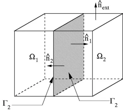
In the case of the non-overlapping domain decomposition, he computational domain,
Ω
, is decomposed into a number of disjoint sub-domains. For the sake of beatify and simplicity only two sub-domains,Ω
1 andΩ
2 will be considered, without any loss of generality. With respect to Fig. 1 the decomposed continuous BVP reads:Given an arbitrary initial value
(
E
1( )0,
E
2( )0)
find(
E
1( )n,
E
2( )n)
through the following iteration ( ) ( ) ( ) ( ) ( ) ( ) ( ) ( ) ( ) ( ) ( ) 2 1 1 1 1 1 1 1 1 1 1 1 1 2 2 2 2 2 1 1 2 1 1 1 1 2 2 2 2 2 2 2 2 2 21
0
in
1
1
ˆ
ˆ
ˆ
ˆ
ˆ
ˆ
on ,
ˆ
ˆ
ˆ
0
on =
\
1
0
in
1
ˆ
ˆ
n n r r n n n n r r n next ext ext ext
n n r r n r
E
k
E
n
E
n
n
E
n
E
n
n
E
n
E
jkn
n
E
E
k
E
n
E
n
ε
µ
α
α
µ
µ
ε
µ
α
µ
− −⎫
∇×
∇×
−
=
Ω
⎪
⎪
⎪
×
∇×
+
× ×
= ×
∇×
−
× ×
Γ
⎬
⎪
⎪
×∇×
+
×
×
=
Γ
∂Ω Γ ⎪
⎭
∇×
∇×
−
=
Ω
×
∇×
+
( ) ( ) ( ) ( ) ( ) 1 1 2 2 1 1 1 `1 1 2 1 2 2 2 21
ˆ
ˆ
ˆ
ˆ
on
ˆ
ˆ
ˆ
0
on =
\
n n n r n next ext ext ext
n
E
n
E
n
n
E
n
E
jkn
n
E
α
µ
− −⎫
⎪
⎪
⎪
× ×
= ×
∇×
−
× ×
Γ
⎬
⎪
⎪
×∇×
+
×
×
=
Γ
∂Ω Γ ⎪
⎭
(2)where
n n
ˆ ˆ
1,
2 andn
ˆ
ext are the unit normal vectors pointing outwards on the interfacesΓ Γ
1,
2 and the exterior boundary, respectively. The parameterα
∈
in the Robin conditions is utilized to optimize the convergence of the algorithm. In this work the optimal conditions derived in [7] are used.C. Mortar method for non-conforming DDM
With the introduction of a dual electric current variable
1
ˆ
,
1, 2
i i i rij
n
E
i
µ
= ×
∇×
=
(3)at interfaces
Γ
1 andΓ
2, the two subdomain problem of (2) decouples into two independent subproblems.( ) ( ) ( ) ( ) ( ) ( ) ( ) 2 1
1
0
in
on ,
1, 2,
ˆ
ˆ
ˆ
0
on =
\
n n i ri i i ri n n n i i i i n next i ext ext i ext i i
E
k
E
j
e
g
i
n
E
jkn
n
E
ε
µ
α
−⎫
∇×
∇×
−
=
Ω
⎪
⎪⎪
−
= −
Γ
⎬
=
⎪
×∇×
+
×
×
=
Γ
∂Ω Γ ⎪
⎪⎭
(4) where(
)
1/ 2ˆ
,
i i i ie
= × ∈
n
E
H
−curl
Γ
(5)is the tangential component of the electric filed in on interface
Γ
i. In addition,( ) ( ) ( ) 1 1 1
,
n n n i neig i neigh ig
−=
j
−−
α
e
− (6)where
neig i
( )
indicates the neighboring domain of domaini
.Before proceeding to the formal weak statement of the BVP, it is necessary to define the following spaces for the primal variables
(
)
{
ˆ
ˆ
ˆ
}
:
;
,
0 ,
ext i=
u
∈
curl
Ω
in
×∇× +
u
jkn n u
× ×
Γ=
X
H
(7)where we have implicitly assume that the bounded polyhedral domain
Ω
has been partitioned intoI
non-overlapping subdomains, namely1
, .
I
i= i k l
k
l
Ω =
∪
Ω
Ω
∩
Ω = ∅
≠
(8)(
)
{
1/ 2}
:
;
.
i ij
div
i − Γ=
∈
Γ
M
H
(9)In this multiple domain setting, the weak statement of the ith decoupled problem of (4) leads to the following saddle point formulation:
Find
(
E
h,
j
h)
∈
X
h×
M
h⊂
X
i×
M
i such that( )
(
)
(
( ))
( )(
)
(
( ))
( ) ( ) 1,
,
,
,
,1
,
,
,
,
neg i n n i h i h h n n n i h i h h ha E
u
b
u
f u
u
i
I
b E
c
j
g
α λ
α
α
λ
λ
−λ
λ
α
Γ⎫
+
=
∀ ∈
∈
⎪ ≤ ≤
⎬
+
=
∀ ∈
∈ ⎪
⎭
X
M
(10)where the bilinear forms
a
i( ) ( )
i i
, ,
b
ii i
, and
c
i( )
i i
,
are given by( )
1
2,
,
i i r ra E u
E
u
k
ε
E udV
µ
Ω=
∫
∇×
i
∇× −
i
(11)( )
,
,
i i h hb
λ
u
j udS
Γ=
∫
i
(12)( )
,
.
i i hc
j
λ
j
λ
dS
Γ=
∫
i
(13)It should be noted here that the Lagrange multiplier
j
h approximates the electric current density on the inter-domain interface. As a result of using a Robin type transmission condition in problem(2), the resulting saddle point formulation of (10) avoids of the zero diagonal block the dual unknowns. The second important point about (10) is the non-conforming nature of the dual part. Non-matching triangulations are allowed on either side of the interface.For the finite element discritization of the saddle point problem(10), second order tetrahedral elements of the 1st Nédélec family are used. The final linear system of equations is of the form
( ) ( 1)
1,
n n i iy
i ii
I
−= +
∀ =
K u
g
(14)where
K u y
i,
i,
i andg
iare of the form,
i i T i i i i T i i⎛
⎞
⎜
⎟
= ⎜
⎟
⎜
⎟
⎝
⎠
A
C
0
K
C
B
D
0
D
T
(15) ( ) ( ) ( ) ( ) ( ) ( ) ( ),
and
,
n i n i n n n i i i i i n n i i⎛
⎞
⎛ ⎞
⎜
⎟
⎛
⎞
⎜ ⎟
=
⎜ ⎟
=
⎜
⎟
=
⎜
⎜
⎟
⎟
⎜
⎟
⎜ ⎟
⎜
⎟
⎝
⎠
⎝ ⎠
⎝
⎠
E
b
e
y
0
u
e
v
j
0
j
(16) ( ) ( ) ( 1) n n i ij j T T n ij ij j −⎛
⎞
⎛
⎞
⎜
⎟
⎜
⎟
=
⎜
⎟
⎜
⎟
=
⎜
⎟
⎜
⎟ ⎜
⎟
⎝
⎠ ⎝
⎠
0
0
0
0
g
0
0
0
0
G j
0
D
T
j
i
(17)note that all matrices involved in (14)-(17) are sparse.
D. DP-FETI like Algorithm
As it was pointed in the introduction, the class of problems we considere have a large number of repeated domains. In a straight forward manner, the solution of (14) would require the solution of every subdomain problem on each iteration step. An elegant way to overcome this is to rewrite (14) as
( ) 1 1 ( )
1,
n n i i i i ii
I
− −=
+
∀ =
u
K y
K g
(18)Before proceeding with the rest of the derivation, let first define two useful restriction operators: one that restrict the solution vector on inter-domain interface unknowns
DP
=
v
R u
(19)and another that restricts into just the dual part of the solution,
.
D
=
j
R u
(20)Applying the surface restriction on both sides of(18) results on
( ) 1 1 ( 1)
.
n n DP i DP i i DP i i − − −=
+
R
u
R
K y
R
K g
(21)Utilizing the well known property of a restriction matrix,
R R
TD D=
I
the following equation is obtained( ) 1 1 ( 1)
,
n T n DP i DP i i DP i D D i − − −=
+
R
u
R
K y
R
K R R g
(22)which can be compactly written as
( ) 0 ( 1)
1,
n n i i i ii
I
−=
+
∀ =
v
x
Z g
(23) where 0 1 1,
,
.
i DP i i DP i D i DP i − −=
=
=
x
R
K y
Z
R
K R
g
R
g
(24) The iteration scheme of (23) can be solved with a Jacobi or Gauss-Seidel stationary iteration method. Note that the iterationmatrix is a dense one, and for its construction require the solution of the subdomain as many times as the dual unknown’s space kernel. Note that the construction of
Z
i is independently of the iteration, thus in can be done once in the preprocessing step. For general domain decomposition this is not efficient way to proceed, but in the case of repeating subdomains the computational cost can be greatly decreased.On the implementation side, the following algorithm summarizes the most import steps of the process.
Algorithm
Let I be the number of domains, K<<I the number of different bounding blocks and mk the number of dual unknowns of block k
Lets denote the row partition of matrices 1
|
2|
|
I i
= ⎣
⎡
M⎤
⎦
Z
z
z
z
and 1|
2|
|
I D= ⎣
⎡
M⎤
⎦
R
r r
r
Pre-Processing for k=1,K assembleK y G
k,
k,
kl,
l
=
neigh k
( )
solveK x
k 0k=
y
k, restrictx
0k=
R
DPx
k0 for mk=1,Mk solve k k k m=
mK z
r
, restrict k k m=
DP mz
R
z
end end Solutionwhile
error
≥
TOL
for i=1,I
initialize
v
i( )n←
x
0i , updateg
i←
G j
il l,
l
=
neigh i
( )
updatev
( )in←
Z
k i( )g
i(n−1) ( ) ( ) ( ) 1 n n i i i n iv
v
e
v
− ∞ ∞−
←
enderror
←
max
( )
e
in
+ +
III. NUMERICAL RESULTS
chosen, the electromagnetic radiation by a 3 different RADAR arrays, and the confinement of light inside photonic crystals, commonly known as photonic band gap (PBG) structures. Through these examples, the convergence, accuracy and computational properties of the proposed method are illustrated.
All examples are unbounded Maxwell’s problems and a first order vector Absorbing Boundary Condition (ABC) were used to approximate the radiation condition. All computations were performed in a PC with single 2.4GHz INTEL XEON processor and 2.0GB RAM. Double precision complex arithmetic is assumed. The computational codes were implemented in object-oriented C++.
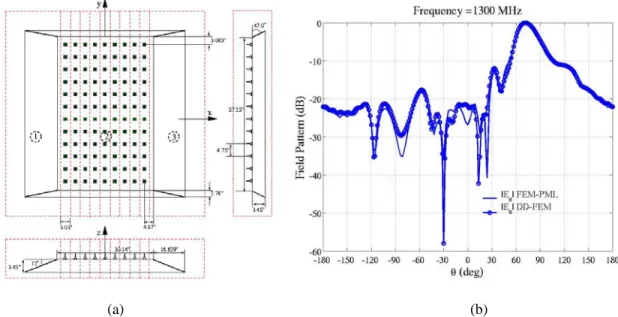
The first antenna radiation considered is shown in Fig. 2(a). It consists of an array of 9×12 monopole radiators excited by a coaxial feeder at their base. The array resides on a finite perfect electric conductor (PEC) plate connected into 4 wedges on each side. The array is excited with constant amplitude and linear progressive phase along the x direction. This excitation ideally results on a radiation peak at the elevation angle
θ
=
90 ,
φ
=
90
, where( )
θ φ
,
are the polar angles with respect toz
ˆ
andx
ˆ
axes. The frequency of operation was assumed
f
=
1.3
GHz
.The configuration is simulated with the proposed method and a full FEM method. In both cases the boundaries of the computational domain are placed
λ
/ 2
away form the structure, whereλ
=
c f
/
is the wavelength in free space. The two main parameters of interest are the shape of the radiation pattern and the directivity of the antenna, which is the ratio of the peak over the total radiated power of the antenna. The x-y cut of the radiation pattern is shown in Fig. 2(b). In the same plot the solid lines represent the full FEM results while the circle/solid line curves represent the proposed method’s results. Much of the dominant component field agrees favorably with the full FEM. At this point it should be noted that the reference full FEM result was obtained using an h-adaptive mesh refinement process with errore
=
5.3%
. Only, some minor discrepancies are present at low level fields. It should be noted that both full FEM and the DDM subdomain solve accuracies were set to 10-3, whereas the outer loop for the DDM was set to 102. For that accuracy, the DDM converged in 32 outer loop iterations.Fig. 2. Antenna array radiation, comparison with full FEM. (a) Top view and cross sections of the monopole antenna array and its mounting structure; the domain partition is denoted with dashed red lines. (b) Far field radiation pattern in the plane x-z, for end-fire excitation.
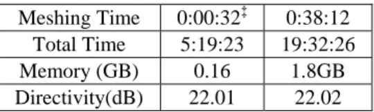
Some more comparisons of the computational effort of the two methods are shown in TABLE I. It is apparent that in every category the proposed DDM outperforms the full FEM. Among the interesting points of this table is the meshing time. In both cases the same mesh generation code was used for the meshing of the geometry. In the full FEM the time indicated is only the time for the creation of an initial mesh of average mesh size of
λ
/ 3
. On the other had, DDM time refers to the total time required to mesh block 1 and block 3 (see Fig. 2) to an average sizeh
=
λ
/ 4
, and fully adaptive mesh refine block 2 to an error ofe
=
2%
.TABLE I COMPARISONS OF THE PROPOSED METHOD AND THE FULL FEM ON A SINGLE 2.4GHZ INTELXEON PROCESSOR PC WITH 2.0GBRAM
DDM FEM
Meshing Time 0:00:32‡ 0:38:12 Total Time 5:19:23 19:32:26 Memory (GB) 0.16 1.8GB Directivity(dB) 22.01 22.02
The second array structure analyzed is the actual array used in the next generation Airborne Early Warning and Control aircrafts (AWACS) RADAR. The array is similar with that of Fig. 2(a) but with 108 monopole elements along the x direction. This is a problem impossible problem to solve with a serial FEM code on any PC. Apart form the memory limitation of a full FEM, one of the toughest hurtle to overcome is the actual meshing of such geometry. Even with the most advanced mesh generation codes of today’s, a problem of this complexity and size will require more than a day for only the initial mesh. With the proposed method, this problem is overcome since it is based on non-matching triangulations on the inter-domain interfaces
The results of the DDM are plotted in Fig. 3. In the left, the electric field distribution is plotted on the surface of the truncation boundary. The strong fields intensities are colored white while small fields are green. On the right of the same figure is depicted the x-y plane of the far-field pattern for both polarizations. The computational domain is approximately
40
λ
×
8
λ
×
2
λ
the total unknown number is 9.22 millions while the dual unknown number is 297.2 thousands. The total memory used was 481MB and the solution time (without preprocessing step) was 15:14sec. The outer loop tolerance was set 10-2, and it was achieved in 30 iterations. It is very interesting to note that for this configuration, this method totally avoids the prepossession step of assemblingk
Z
since it was once for all obtained in the solution of the previous example. This appealing future makes the method very suitable for design and optimization.Fig. 3. Radiation by a 108×12 element array monopole. (a) Electric filed on the surface of the computational domain. (b) Far-Field radiation pattern in x-z plane.
To briefly introduce a comparison the proposed method with the direct version of the domain decomposition described by equation(14), another array radiation example was considered. This time the array was a planar one, under broadside excitation
θ
=
0
. The array elements are “Vivaldi” tapered slot antennas, as it is illustrated in various view on Fig. 4(a). In the right side of the same figure a 50×50 array configuration is depicted. The most important results of the simulations are tabulated in TABLE II. The computational effort required for the proposed method is significantly smaller than the direct domain decomposition. Moreover, both methods resulted in an exactly same answer of the far-field pattern.‡ The time includes the mesh of blocks 1 and 3, and, a full h-adaptive mesh refinement solution process for block 2, the error was set to 2% (a) (b)
Fig. 4. Radiation by the “Vivaldi” array. (a) Geometry, excitation and materials of the Vivaldi antenna element. (b) Current distribution of the metallic parts of the array and the superimposed far-field radiation pattern on the circular plate on the top of the array.
TABLE IICOMPARISON OF DIRECT DDM WITH PROPOSED METHOD FOR VARIOUS SIZES OF THE VIVALDI ARRAY
Array Size Total Unknown Number Memory(MB) Direct DD Time Direct DD Memory(MB) Proposed Time Proposed DD 3×3 98K 11 00:04:00 16 00:08:00 7×7 534K 17 00:25:00 17.7 00:08:00 50×50 27,230K 471 30:12:00 55.6 00:28:00 100×100 108,900K 1,650 112:40:00 167 01:27:00 300×300 980,100K - - 1,370 12:23:00
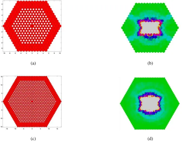
The next application is borrowed for the optics and lightwave technology. As it is shown in Fig. 5 a GaAs substrate is drilled with air holes on a triangular stencil. These holes at certain frequency bands act like barriers, so the light can not propagate through the structure. In the center of the substrate, a single defect is created by living the substrate intact. This forms a nanocavity that traps the light inside. This particular arrangement is widely used in laser technology. In this example it will be shown that the trapping of the light gets more and more effective as the number of air hole layers around the nanocavity increases. Unfortunately, this increases the computational domain size, thus the memory and time requirements. The present method is ideal for analyzing this type of problems, since the preprocessing cost is paid only once, regardless of the number of layers around the nanocavity.
Fig. 5. A Laser nanocavity surrounded by a 2 dimensional photonic crystal. (a) Geometry, material and excitation configuration. (b) Electric filed distribution at the mid-plane (x-y) of the geometry.
The electric field distributions on the transverse mid plane of the substrante is plotted in Fig. 5(b),Fig. 6(b) and (d) for 3, 7 (a) (b)
and 14 layers nanocavities. It is clear that the field is trapped tighter and tighter as the number of air layers increases.
Fig. 6. Top view and field distribution of more realistic nanocavities. (a) A 7 layer PBG nanocavity, top view. (b) Electric field distribution on the transverse mid-plane (x-y) of the 7 layer PBG nanocavity. (c) A 14 layer PBG nanocavity, top view. (d) Electric filed distribution of the x-y plane of the 14 layer PPB nanocavity.
TABLE IIICOMPUTATIONAL STATISTICS OF THE PORPOSED METHOD FOR THE PBG NANOCAVITY EXAMPLES.THE COMPUTATIONS WERE PREFORMED ON A SINGEL
2.4GHZ INTELXEON PROCESSORE WITH 2GB RAM.
Layers Domains Dual Total Memory Z time Solve time
3 127 29.9K 510.1K 131.48MB 0:31:25 0:01:07 (49)
7 331 78.1K 2,252.1K 142.54MB 0:31:25 0:06:22 (138)
14 919 216.8K 8,365.7K 156.02MB 0:31:25 7:12:41 (294)
IV. CONCLUSIONS
This paper introduced an efficient method for analyzing large electromagnetic and optic problems that exhibit spatial repetitions. The method was based on three core ingredients: First an optimized Robin type transmission condition was used to speed up the convergence of the outer iteration loop of the non-overlapping Schwarz algorithm. A non-conforming mortar like formulation was implemented to relax the mesh generation, and avid periodic meshes. Thirdly, an efficient algorithm was used to significantly speed up the computation per outer loop iteration. Some results on complex large scale real life industrial problems were used to illustrate the efficiency of the method.
REFERENCES
[1] B. Després “Méthodes de décomposition de domaine pour les problémes de propagation d’ondes en régime harmonique”, Ph.D dissertation Paris, 1991 [2] J-D Benamou, and B. Desprès, “A domain decomposition method for the Helmholtz equation and related optimal control problems”, J.Comput. Phys.., vol
136, pp. 68-82. 1997.
[3] F. Collino, G Delbue, P. Joly, and A Piacentini, “A new interface condition in the non-overlapping domain decomposition method for the Maxwell equations”, Comput. Methods Appl. Mech. Engrg., vol 148, pp. 195-207, 1997.
[4] A. Piacentini, and N. Rosa, “An improved domain decomposition method for the 3D Helmholtz equation”, Comput. Methods Appl. Mech. Engrg., vol 162, pp. 113-124, 1998.
[5] B. Stupfel, “A fast-domain decomposition method for the solution of electromagnetic scattering by large objects”, IEEE Trans. Antennas Propagat., vol 44, no. 10, pp. 1375-1385, Oct. 1996.
(a) (b)
[6] B. Stupfel, and Martine Mognot “A domain decomposition method for the vector wave equation”, IEEE Trans. Antennas Propagat., vol 48, no. 5, pp. 653-660, May. 2000.
[7] M. Gander, F. Magoulès, and F. Nataf “Optimized Schwarz methods without overlap for the Helmholtz equation”, SIAM J. Scir. Comput., vol. 24, no 1, pp. 38-60, 2002.
[8] M. Gander, L. Halpern, and F. Nataf “Optimized Schwarz methods”, in Proceedings of the 12the International Conf. on Domain Decomp. Methods., Chiba, Japan, 2001, pp. 15-26.
[9] M. Gander, “Optimized Schwarz methods for Helmholtz Problems”, in Proceedings of the 12the International Conf. on Domain Decomp. Methods., Chiba, Japan, 2002 , pp. 245-252.
[10] C. Farhat, and F.-X. Raux, “A method of finite element tearing and interconnecting and its parallel solution algorithm,”Internat. J. Numer. Meth. Eng., vol. 32, pp. 1205 –1227, 1991.
[11] B. I. Wohlmuth Discretization Methods and Iterative Solvers Based on Domain Decomposition, Berlin: Springer-Verlag, 2001 [12] L. F. Pavarino and A. Toselli, Recent Developments in Domain Decomposition Methods, Berlin: Springer-Verlag, 2002.