A primal-dual algorithm for group sparse
regularization with overlapping groups
Sofia Mosci DISI- Universit`a di Genova [email protected]
Silvia Villa DISI- Universit`a di Genova [email protected]
Alessandro Verri DISI- Universit`a di Genova [email protected]
Lorenzo Rosasco IIT - MIT [email protected]
Abstract
We deal with the problem of variable selection when variables must be selected group-wise, with possibly overlapping groups defined a priori. In particular we propose a new optimization procedure for solving the regularized algorithm pre-sented in [12], where the group lasso penalty is generalized to overlapping groups of variables. While in [12] the proposed implementation requires explicit repli-cation of the variables belonging to more than one group, our iterative procedure is based on a combination of proximal methods in the primal space and projected Newton method in a reduced dual space, corresponding to the active groups. This procedure provides a scalable alternative with no need for data duplication, and allows to deal with high dimensional problems without pre-processing for dimen-sionality reduction. The computational advantages of our scheme with respect to state-of-the-art algorithms using data duplication are shown empirically with numerical simulations.
1
Introduction
Sparsity has become a popular way to deal with small samples of high dimensional data and, in a broad sense, refers to the possibility of writing the solution in terms of a few building blocks. Often, sparsity based methods are the key towards finding interpretable models in real-world problems. In particular, regularization based on`1type penalties is a powerful approach for dealing with the
prob-lem of variable selection, since it provides sparse solutions by minimizing a convex functional. The success of`1regularization motivated exploring different kinds of sparsity properties for
(general-ized) linear models, exploiting available a priori information, which restricts the admissible sparsity patterns of the solution. An example of a sparsity pattern is when the input variables are partitioned into groups (known a priori), and the goal is to estimate a sparse model where variables belonging to the same group are either jointly selected or discarded. This problem can be solved by regularizing with the group-`1penalty, also known as group lasso penalty, which is the sum, over the groups, of
the euclidean norms of the coefficients restricted to each group.
A possible generalization of group lasso is to consider groups of variables which can be potentially overlapping, and the goal is to estimate a model which support is the union of groups. This is a common situation in bioinformatics (especially in the context of high-throughput data such as gene expression and mass spectrometry data), where problems are characterized by a very low number of samples with several thousands of variables. In fact, when the number of samples is not sufficient to guarantee accurate model estimation, an alternative is to take advantage of the huge amount of prior knowledge encoded in online databases such as the Gene Ontology. Largely motivated by ap-plications in bioinformatics, a new type of penalty is proposed in [12], which is shown to give better
performances than simple`1regularization.
A straightforward solution to the minimization problem underlying the method proposed in [12] is to apply state-of-the-art techniques for group lasso (we recall interior-points methods [3, 20], block coordinate descent [16], and proximal methods [9, 21], also known as forward-backward splitting algorithms, among others) in an expanded space, built by duplicating variables that belong to more than one group.
As already mentioned in [12], though very simple, such an implementation does not scale to large datasets, when the groups have significant overlap, and a more scalable algorithm with no data du-plication is needed. For this reason we propose an alternative optimization approach to solve the group lasso problem with overlap. Our method does not require explicit replication of the features and is thus more appropriate to deal with high dimensional problems with large groups overlap. Our approach is based on a proximal method (see for example [18, 6, 5]), and two ad hoc results that allow to efficiently compute the proximity operator in a much lower dimensional space: with Lemma 1 we identify the subset ofactivegroups, whereas in Theorem 2 we formulate the reduced dual problem for computing the proximity operator, where the dual space dimensionality coincides with the number of active groups. The dual problem can then be solved via Bertsekas’ projected Newton method [7]. We recall that a particular overlapping structure is the hierarchical structure, where the overlap between groups is limited to inclusion of a descendant in its ancestors. In this case the CAP penalty [24] can be used for model selection, as it has been done in [2, 13], but ancestors are forced to be selected when any of their descendant are selected. Thanks to the nested structure, the proximity operator of the penalty term can be computed exactly in a finite number of steps [14]. This is no longer possible in the case of general overlap. Finally it is worth noting that the penalty analyzed here can be applied also to hierarchical group lasso. Differently from [2, 13] selection of ancestors is no longer enforced.
The paper is organized as follows. In Section 2 we recall the group lasso functional for overlap-ping groups and set some notations. In Section 3 we state the main results, present a new iterative optimization procedure, and discuss computational issues. Finally in Section 4 we present some numerical experiments comparing running time of our algorithm with state-of-the-art techniques. The proofs are reported in the Supplementary material.
2
Problem and Notations
We first fix some notations. Given a vectorβ ∈Rd, whilek·kdenotes the`
2-norm, we will use the
notationkβkG = (P
j∈Gβ
2
j)
1/2to denote the`
2-norm of the components ofβinG⊂ {1, . . . , d}.
Then, for any differentiable functionf : RB →
R, we denote by∂rf its partial derivative with
respect to variablesr, and by∇f = (∂rf)Br=1its gradient.
We are now ready to cast group`1 regularization with overlapping groups as the following
varia-tional problem. Given a training set{(xi, yi)ni=1} ∈(X×Y)
n, a dictionary(ψ
j)dj=1, andBsubsets
of variablesG ={Gr}Br=1withGr ⊂ {1, . . . , d}, we assume the estimator to be described by a
generalized linear modelf(x) =Pd
j=1ψj(x)βjand consider the following regularization scheme
β∗= argmin β∈Rd Eτ(β) = argmin β∈Rd 1 nkΨβ−yk 2 + 2τΩGoverlap(β) , (1)
whereΨis then×dmatrix given by the featuresψjin the dictionary evaluated in the training set
points,[Ψ]i,j =ψj(xi). The term n1kΨβ−yk
2
is the empirical error, n1Pn
i=1`(f(xi), yi), when
the cost function1`:R×Y →R+is the square loss,`(f(x), y) = (y−f(x))2.
The penalty termΩGoverlap :Rd →R+ is lower semicontinuous, convex, and one-homogeneous, (ΩGoverlap(λβ) =λΩGoverlap(β),∀β∈Rdandλ∈R+), and is defined as
ΩGoverlap(β) = inf (v1,...,vB),vr∈Rd,supp(vr)⊂Gr,PBr=1vr=β B X r=1 kvrk.
The functional ΩGoverlap was introduced in [12] as a generalization of the group lasso penalty to allow overlapping groups, while maintaining the group lasso property of enforcing sparse solutions which support is aunion of groups. When groups do not overlap,ΩGoverlapreduces to the group lasso
1
penalty. Note that, as pointed out in [12], usingPB
r=1kβkGr as generalization of the group lasso
penalty leads to a solution which support is thecomplement of the union of groups. For an extensive study of the properties ofΩGoverlap, its comparison with the`1norm, and its extension to graph lasso,
we therefore refer the interested reader to [12].
3
The GLO-pridu Algorithm
If one needs to solve problem (1) for high dimensional data, the use of standard second-order meth-ods such as interior-point methmeth-ods is precluded (see for instance [6]), since they need to solve large systems of linear equations to compute the Newton steps. On the other hand, first order methods inspired to Nesterov’s seminal paper [19] (see also [18]) and based on proximal methods already proved to be a computationally efficient alternative in many machine learning applications [9, 21]. 3.1 A Proximal algorithm
Given the convex functionalEτin (1), which is sum of a differentiable term, namely n1kΨβ−yk
2
, and a non-differentiable one-homogeneous term 2τΩGoverlap, its minimum can be computed with following acceleration of the iterative forward-backward splitting scheme
βp= I−πτ /σK hp− 1 nσΨ T(Ψhp−y) cp= (1−tp)cp−1, tp+1= −cp+ q c2 p+ 8cp /4 (2) hp+1=βp(1−tp+1+ tp+1 tp ) +βp−1(tp−1) tp+1 tp
for a suitable choice ofσ. Due to one-homogeneity ofΩGoverlap, the proximity operator associated to τσΩGoverlapreduces to the identity minus the projection onto the subdifferential of τσΩGoverlapat the origin, which is a closed and convex set. We will denote such a projection asπτ /σK, where
K=∂ΩGoverlap(0). The above scheme is inspired to [10], and is equivalent to the algorithm named FISTA [5], which convergence is guaranteed, as recalled in the following theorem
Theorem 1 Givenβ0∈
Rd, andσ=||ΨTΨ||/n, leth1=β0andt1= 1, c0= 1, then there exists a constantC0such that the iterative update(10)satisfies
Eτ(βp)− Eτ(β∗)≤
C0
p2. (3)
As it happens for other accelerations of the basic forward-backward splitting algorithm such as [19, 6, 4], convergence of the sequenceβp is no longer guaranteed unless strong convexity is assumed. However, sacrificing theoretical convergence for speed may be mandatory in large scale applications. Furthermore, there is a strong empirical evidence thatβpis indeed convergent (see Section 4).
3.2 The projection
Note that the proximity operator of the penaltyΩGoverlapdoes not admit a closed form and must be computed approximatively. In fact the projection on the convex set
K=∂ΩGoverlap(0) ={v∈Rd,kvkGr≤1forr= 1, . . . , B}.
cannot be decomposed group-wise, as in standard group`1regularization, which proximity operator
resolves to a group-wise soft-thresholding operator (see Eq. (9) later). Nonetheless, the following lemma shows that, when evaluating the projection, πK, we can restrict ourselves to a subset of
ˆ
B =|G| ≤ˆ Bactivegroups. This equivalence is crucial for speeding up the algorithm, in factBˆis the number of selected groups which is small if one is interested in sparse solutions.
Lemma 1 Givenβ ∈Rd,G ={Gr}Br=1withGr⊂ {1, . . . , d}, andτ >0, the projection onto the
convex setτ KwithK={v∈Rd,kvkGr≤1forr= 1, . . . , B}is given by
Minimize kv−βk2
subject to v∈Rd,kvkG≤τforG∈G.ˆ
(4)
The proof (given in the supplementary material) is based on the fact that the convex setτ Kis the intersection of cylinders that are all centered on a coordinate subspace. SinceBˆ is typically much smaller thand, it is convenient to solve the dual problem associated to (4).
Theorem 2 Givenβ ∈ Rd,{G
r}Br=1 withGr ⊂ {1, . . . , d}, andτ > 0, the projection onto the
convex setτ KwithK={v∈Rd,kvkGr≤τforr= 1, . . . , B}is given by
[πτ K(β)]j=
βj
(1 +PBˆ
r=1λ∗r1r,j)
forj= 1, . . . , d (5)
whereλ∗is the solution of
argmax λ∈RB+ˆ f(λ), withf(λ) := d X j=1 −β2 j 1 +PBˆ r=11r,jλr − ˆ B X r=1 λrτ2, (6) ˆ
G={G∈ G, kβkG> τ}:={Gˆ1, . . . ,GˆBˆ}, and1r,jis1ifjbelongs to groupGˆrand0otherwise.
Equation (6) is the dual problem associated to (4), and, since strong duality holds, the minimum of (4) is equal to the maximum of the dual problem, which can be efficiently solved via Bertsekas’ projected Newton method described in [7], and here reported as Algorithm 1.
Algorithm 1Projection Given:β ∈Rd, λinit∈RBˆ, η∈(0,1), δ∈(0,1/2), >0 Initialize:q= 0, λ0=λinit while(∂rf(λq)>0ifλqr= 0,or|∂rf(λq)|> ifλqr>0,forr= 1, . . . ,B)ˆ do q:=q+ 1 q =min{,||λq−[λq− ∇f(λq)]+||} I+q ={r such that 0≤λqr≤q, ∂rf(λq)>0} Hr,s = 0 ifr6=s,andr∈ I+qors∈ I q + ∂r∂sf(λq) otherwise (7) λ(α) = [λq−α(Hq)−1∇f(λq)]+ m= 0 while f(λq)−f(λ(ηm))≥δnηmP r /∈Iq +∂rf(λ q) +P r∈Iq +∂rf(λ q)[λq r−λr(ηm)] o do m:=m+ 1 end while λq+1=λ(ηm) end while return λq+1
Bertsekas’ iterative scheme combines the basic simplicity of the steepest descent iteration [22] with the quadratic convergence of the projected Newton’s method [8]. It does not involve the solution of a quadratic program thereby avoiding the associated computational overhead.
3.3 Computing the regularization path
In Algorithm 2 we report the completeGroupLasso withOverlapprimal-dual (GLO-pridu) scheme for computing the regularization path, i.e. the set of solutions corresponding to different values of the regularization parameterτ1> . . . > τT, for problem (1). Note that we employ thecontinuation
strategy proposed in [11]. A similar warm starting is applied to the inner iteration, where at thep-th stepλinitis determined by the solution of the(p−1)-th projection. Such an initialization empirically proved to guarantee convergence, despite the local nature of Bertsekas’ scheme.
3.4 The replicates formulation
An alternative way to solve the optimization problem (1) is proposed by [12], where the authors show that problem (1) is equivalent to the standard group`1regularization (without overlap) in an
Algorithm 2GLO-pridu regularization path Given:τ1> τ2>· · ·> τT,G, η∈(0,1), δ∈(0,1/2), 0>0, ν >0 Let:σ=||ΨTΨ||/n Initialize:β(τ0) = 0 fort= 1, . . . , T do Initialize:β0=β(τt−1), λ∗0= 0 while||βp−βp−1||> ν||βp−1||do •w=hp−(nσ)−1ΨT(Ψhp−y) • FindGˆ={G∈ G,kwkG≥τ}
• Computeλ∗pvia Algorithm 1 with groupsG, initializationˆ λ∗p−1and tolerance0p−3/2
• Computeβpasβjp=wj(1 +P
ˆ
B r=1λ
q+1
r 1r,j)−1forj= 1, . . . , d, see Equation (5)
• Updatecp, tp, andhpas in (10) end while β(τt) =βp end for return β(τ1), . . . , β(τT) ˜ β∗∈argmin ˜ β∈Rd˜ ( 1 n|| ˜ Ψ ˜β−y||2+ 2τ B X r=1 ||β||˜ G˜r ) , (8)
whereΨ˜ is the matrix built by concatenating copies ofΨrestricted each to a certain group, i.e. ( ˜Ψj)j∈G˜r = (Ψj)j∈Gr, where{G˜1, . . . ,G˜B}={[1, . . . ,|G1|],[1+|G1|, . . . ,|G1|+|G2|], . . . ,[ ˜d−
|GB|, . . . ,d|˜]}, andd˜= P B
r=1|Gr| is the number of total variables obtained after including the
replicates. One can then reconstructβ∗fromβ˜∗asβj∗ =PB
r=1φGr( ˜β ∗), whereφ Gr :R ˜ d → Rd
mapsβ˜inv∈Rd, such that supp(v)⊂Grand(vj)j∈Gr = ( ˜βj)j∈G˜r, forr= 1, . . . , B. The main
advantage of the above formulation relies on the possibility of using any state-of-the-art optimization procedure for group lasso. In terms of proximal methods, a possible solution is given by Algorithm 3, whereSτ /σis the proximity operator of the new penalty, and can be computed exactly as
Sτ /σ( ˜β) j =||β˜||G˜ r− τ σ + ˜ βj, forj∈G˜r, forr= 1, . . . , B. (9) Algorithm 3GL-prox Given:β˜0∈ Rd, τ >0, σ=||Ψ˜TΨ˜||/n Initialize:p= 0,˜h1= ˜β0, t1= 1
whileconvergence not reacheddo p:=p+ 1 ˜ βp=Sτ /σ ˜ hp−(nσ)−1Ψ˜T( ˜Ψ˜hp−y) (10) cp= (1−tp)cp−1, tp+1= 1 4(−cp+ q c2 p+ 8cp) ˜ hp+1= ˜βp(1−tp+1+ tp+1 tp ) + ˜βp−1(tp−1) tp+1 tp end while return β˜p
Note that in principle, by applying Lemma 1, the group-soft-thresholding operator in (9) can be com-puted only on the active groups. In practice this does not yield any advantage, since the identification of the active groups has the same computational cost of the thresholding itself.
3.5 Computational issues
For both GL-prox and GLO-pridu, the complexity of one iteration is the sum of the complexity of computing the gradient of the data term and the complexity of computing the proximity operator of the penalty term. The former has complexityO(dn)andO( ˜dn)for GLO-pridu and GL-prox,
respectively, for the casen < d. One should then add at each iteration, the cost of performing the projection ontoK. This can be neglected for the case of replicated variables.On the other hand, the time complexity of one iteration for Algorithm 1 is driven by the number of active groupsB.ˆ This number is typically small when looking for sparse solutions. The complexity is thus given by the sum of the complexity of evaluating the inverse of theBˆ ×Bˆ matrixH,O( ˆB3), and the
complexity of performing the productH−1∇g(λ),O( ˆB2). The worst case complexity would then
be O( ˆB3). Nevertheless, in practice the complexity is much lower because matrix H is highly sparse. In fact, Equation (7) tells us that the part of matrixH corresponding to the active setI+is
diagonal. As a consequence, ifBˆ = ˆB−+ ˆB+, whereBˆ− is the number of non active constraints,
andBˆ+is the number of active constraints, then the complexity of inverting matrixH is at most
O( ˆB+) +O( ˆB−3). Furthermore theBˆ−×Bˆ−non diagonal part of matrixH is highly sparse, since
Hr,s = 0ifGˆr∩G˜s=∅and the complexity of inverting it is in practice much lower thanO( ˆB−3).
The worst case complexity for computing the projection ontoKis thusO(q·Bˆ+) +O(q·Bˆ−3),
whereqis the number of iterations necessary to reach convergence. Note that even if, in order to guarantee convergence, the tolerance for evaluating convergence of the inner iteration must decrease with the number of external iterations, in practice, thanks to warm starting, we observed thatqis rarely greater than 10 in the experiments presented here.
Concerning the number of iterations required to reach convergence for GL-prox in the replicates formulation, we empirically observed that it requires a much higher number of iterations than GLO-pridu (see Table 3). We argue that such behavior is due to the combination of two occurences: 1) the local condition number of matrixΨ˜ is 0 even ifΨis locally well conditioned, 2) the decomposition of β∗ as β˜∗ is possibly not unique, which is required in order to have a unique solution for (8). The former is due to the presence of replicated columns inΨ˜. In fact, sinceEτ is convex but not
necessarily strictly convex – as whenn < d–, uniqueness and convergence is not always guaranteed unless some further assumption is imposed. Most convergence results relative to`1regularization
link uniqueness of the solution as well as the rate of convergence of the Soft Thresholding Iteration to some measure of local conditioning of the Hessian of the differentiable part ofEτ(see for instance
Proposition 4.1 in [11], where the Hessian restricted to the set of relevant variables is required to be full rank). In our case the Hessian for GL-prox is simplyH˜ = 1/nΨ˜TΨ˜, so that, if the relevant groups have non null intersection, thenH˜ restricted to the set of relevant variables is by no means full rank. Concerning the latter argument, we must say that in many real world problems, such as bioinformatics, one cannot easily verify that the solution indeed has a unique decomposition. In fact, we can think of trivial examples where the replicates formulation has not a unique solution.
4
Numerical Experiments
In this section we present numerical experiments aimed at comparing the running time performance of GLO-pridu with state-of-the-art algorithms. To ensure a fair comparison, we first run some pre-liminary experiments to identify the fastest codes for group`1regularization with no overlap. We
refer to [6] for an extensive empirical and theoretical comparison of different optimization proce-dures for solving`1regularization. Further empirical comparisons can be found in [15].
4.1 Comparison of different implementations for standard group lasso
We considered three algorithms which are representative of the optimization techniques used to solve group lasso: interior-point methods, (group) coordinate descent and its variations, and prox-imal methods. As an instance of the first set of techniques we employed the publicly available Matlab code at http://www.di.ens.fr/˜fbach/grouplasso/index.htm described in [1]. For coordinate descent methods, we employed the R-packagegrlplasso, which imple-ments block coordinate gradient descent minimization for a set of possible loss functions. In the following we will refer to these two algorithms as “’GL-IP” and “GL-BCGD”. Finally we use our Matlab implementation of Algorithm GL-prox as an instance of proximal methods.
We first observe that the solutions of the three algorithms coincide up to an error which depends on each algorithm tolerance. We thus need to tune each tolerance in order to guarantee that all iterative algorithms are stopped when the level of approximation to the true solution is the same.
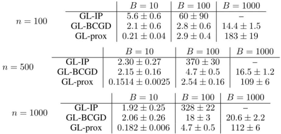
Table 1: Running time (mean and standard deviation) in seconds for computing the entire regular-ization path of GL-IP, GL-BCGD, and GL-prox for different values ofB, andn. ForB = 1000, GL-IP could not be computed due to memory reasons.
n= 100 B= 10 B= 100 B= 1000 GL-IP 5.6±0.6 60±90 – GL-BCGD 2.1±0.6 2.8±0.6 14.4±1.5 GL-prox 0.21±0.04 2.9±0.4 183±19 n= 500 B= 10 B= 100 B= 1000 GL-IP 2.30±0.27 370±30 – GL-BCGD 2.15±0.16 4.7±0.5 16.5±1.2 GL-prox 0.1514±0.0025 2.54±0.16 109±6 n= 1000 B= 10 B= 100 B= 1000 GL-IP 1.92±0.25 328±22 – GL-BCGD 2.06±0.26 18±3 20.6±2.2 GL-prox 0.182±0.006 4.7±0.5 112±6
Toward this end, we run Algorithm GL-prox with machine precision,ν = 10−16, in order to have
a good approximation of the asymptotic solution. We observe that for many values ofnandd, and over a large range of values ofτ, the approximation of GL-prox when ν= 10−6 is of the same order of the approximation of GL-IP withoptparam.tol= 10−9, and of GL-BCGD withtol= 10−12. Note also that with these tolerances the three solutions coincide also in terms of selection, i.e. their supports are identical for each value ofτ. Therefore the following results correspond to optparam.tol= 10−9 for GL-IP,tol= 10−12for GL-BCGD, and ν = 10−6for GL-prox. For the other parameters of GL-IP we used the values used in the demos supplied with the code. Concerning the data generation protocol, the input variablesx= (x1, . . . , xd)are uniformly drawn
from[−1,1]d. The labelsyare computed using a noise-corrupted linear regression function, i.e.y=
β·x+w, whereβdepends on the first30variables,βj = 1ifj= 1, . . . ,30, and0otherwise,wis an
additive gaussian white noise, and the signal to noise ratio is 5:1. In this case the dictionary coincides with the variables,Ψj(x) =xj forj= 1, . . . , d. We then evaluate the entire regularization path for
the three algorithms withBsequential groups of10variables, (G1=[1, . . . ,10],G2=[11, . . . ,20],
and so on), for different values ofnandB. In order to make sure that we are working on the correct range of values for the parameterτ, we first evaluate the set of solutions of GL-prox corresponding to a large range of 500 values forτ, withν = 10−4. We then determine the smallest value ofτ
which corresponds to selecting less thannvariables,τmin, and the smallest one returning the null
solution,τmax. Finally we build the geometric series of50values betweenτminandτmax, and use
it to evaluate the regularization path on the three algorithms. In order to obtain robust estimates of the running times, we repeat 20 times for each pairn, B.
In Table 1 we report the computational times required to evaluate the entire regularization path for the three algorithms. Algorithms GL-BCGD and GL-prox are always faster than GL-IP which, due to memory reasons, cannot by applied to problems with more than5000variables, since it requires to store the d×dmatrixΨT ×Ψ. It must be said that the code for GP-IL was made available
mainly in order to allow reproducibility of the results presented in [1], and is not optimized in terms of time and memory occupation. However it is well known that standard second-order methods are typically precluded on large data sets, since they need to solve large systems of linear equations to compute the Newton steps. GL-BCGD is the fastest for B = 1000, whereas GL-prox is the fastest forB = 10,100. The candidates as benchmark algorithms for comparison with GLO-pridu are GL-prox and GL-BCGD. Nevertheless we observed that, when the input data matrix contains a significant fraction of replicated columns, this algorithm does not provide sparse solutions. We therefore compare GLO-pridu with GL-prox only.
4.1.1 Projection vs duplication
The data generation protocol is equal to the one described in the previous experiments, butβdepends on the first12/5bvariables (which correspond to the first three groups)
β = (c, . . . , c | {z } b·12/5times ,0, 0, . . . , 0 | {z } d−b·12/5times ).
We then defineBgroups of sizeb, so thatd˜=B·b > d. The first three groups correspond to the subset of relevant variables, and are defined asG1 = [1, . . . , b],G2 = [4/5b+ 1, . . . ,9/5b], and
G3= [1, . . . , b/5,8/5b+ 1, . . . ,12/5b], so that they have a20%pair-wise overlap. The remaining
B −3 groups are built by randomly drawing sets ofb indexes from[1, d]. In the following we will letn= 10|G1∪G2∪G3|, i.e. nis ten times the number of relevant variables, and varyd, b.
We also vary the number of groupsB, so that the dimension of the expanded space isαtimes the input dimension,d˜= αd, withα = 1.2,2,5. Clearly this amounts to takingB = α·d/b. The parameterαcan be thought of as the average number of groups a single variable belongs to. We identify the correct range of values forτas in the previous experiments, using GLO-pridu with loose tolerance, and then evaluate the running time and the number of iterations necessary to compute the entire regularization path for GL-prox on the expanded space and GLO-pridu, both withν= 10−6. Finally we repeat 20 times for each combination of the three parametersd, b, andα.
Table 2: Running time (mean±standard deviation) in seconds forb= 10(top), andb= 100(below). For eachdandα, the left and right side correspond to GLO-pridu, and GL-prox, respectively.
α= 1.2 α= 2 α= 5 d=1000 0.15±0.04 0.20±0.09 1.6±0.9 5.1±2.0 12.4±1.3 68±8 d=5000 1.1±0.4 1.0±0.6 1.55±0.29 2.4±0.7 103±12 790±57 d=10000 2.1±0.7 2.1±1.4 3.0±0.6 4.5±1.4 460±110 2900±400 α= 1.2 α= 2 α= 5 d=1000 11.7±0.4 24.1±2.5 11.6±0.4 42±4 13.5±0.7 1467±13 d=5000 31±13 38±15 90±5 335±21 85±3 1110±80 d=10000 16.6±2.1 13±3 90±30 270±120 296±16 –
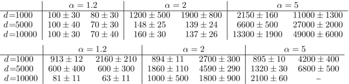
Table 3: Number of iterations (mean±standard deviation) forb= 10(top) andb = 100(below). For eachdandα, the left and right side correspond to GLO-pridu, and GL-prox, respectively.
α= 1.2 α= 2 α= 5 d=1000 100±30 80±30 1200±500 1900±800 2150±160 11000±1300 d=5000 100±40 70±30 148±25 139±24 6600±500 27000±2000 d=10000 100±30 70±40 160±30 137±26 13300±1900 49000±6000 α= 1.2 α= 2 α= 5 d=1000 913±12 2160±210 894±11 2700±300 895±10 4200±400 d=5000 600±400 600±300 1860±110 4590±290 1320±30 6800±500 d=10000 81±11 63±11 1000±500 1800±900 2100±60 –
Running times and number of iterations are reported in Table 2 and 3, respectively. When the degree of overlap αis low the computational times of GL-prox and GLO-pridu are comparable. Asα increases, there is a clear advantage in using GLO-pridu instead of GL-prox. The same behavior occurs for the number of iterations.
5
Discussion
We have presented an efficient optimization procedure for computing the solution of group lasso with overlapping groups of variables, which allows dealing with high dimensional problems with large groups overlap. We have empirically shown that our procedure has a great computational advantage with respect to state-of-the-art algorithms for group lasso applied on the expanded space built by replicating variables belonging to more than one group. We also mention that computational performance may improve if our scheme is used as core for the optimization step of active set methods, such as [23]. Finally, as shown in [17], the improved computational performance enables to use group`1regularization with overlap for pathway analysis of high-throughput biomedical data,
since it can be applied to the entire data set and using all the information present in online databases, without pre-processing for dimensionality reduction.
References
[1] F. Bach. Consistency of the group lasso and multiple kernel learning. Journal of Machine Learning Research, 9:1179–1225, 2008.
[2] F. Bach. High-dimensional non-linear variable selection through hierarchical kernel learning. Technical Report HAL 00413473, INRIA, 2009.
[3] F. R. Bach, G. Lanckriet, and M. I. Jordan. Multiple kernel learning, conic duality, and the smo algorithm. InICML, volume 69 ofACM International Conference Proceeding Series, 2004. [4] A. Beck and Teboulle. M. Fast gradient-based algorithms for constrained total variation image
denoising and deblurring problems. IEEE Transactions on Image Processing, 18(11):2419– 2434, 2009.
[5] A. Beck and M. Teboulle. A fast iterative shrinkage-thresholding algorithm for linear inverse problems. SIAM J. Imaging Sci., 2(1):183–202, 2009.
[6] S. Becker, J. Bobin, and E. Candes. Nesta: A fast and accurate first-order method for sparse recovery, 2009.
[7] D. Bertsekas. Projected newton methods for optimization problems with simple constraints.
SIAM Journal on Control and Optimization, 20(2):221–246, 1982.
[8] R. Brayton and J. Cullum. An algorithm for minimizing a differentiable function subject to. J. Opt. Th. Appl., 29:521–558, 1979.
[9] J. Duchi and Y. Singer. Efficient online and batch learning using forward backward splitting.
Journal of Machine Learning Research, 10:28992934, December 2009.
[10] O. Guler. New proximal point algorithm for convex minimization. SIAM J. on Optimization, 2(4):649–664, 1992.
[11] E. T. Hale, W. Yin, and Y. Zhang. Fixed-point continuation for l1-minimization: Methodology and convergence. SIOPT, 19(3):1107–1130, 2008.
[12] L. Jacob, G. Obozinski, and J.-P. Vert. Group lasso with overlap and graph lasso. InICML, page 55, 2009.
[13] R. Jenatton, J.-Y . Audibert, and F. Bach. Structured variable selection with sparsity-inducing norms. Technical report, INRIA, 2009.
[14] R. Jenatton, J. Mairal, G. Obozinski, and F. Bach. Proximal methods for sparse hierarchical dictionary learning. InProceeding of ICML 2010, 2010.
[15] I. Loris. On the performance of algorithms for the minimization ofl1-penalized functionals. Inverse Problems, 25(3):035008, 16, 2009.
[16] L. Meier, S. van de Geer, and P. Buhlmann. The group lasso for logistic regression. J. R. Statist. Soc, B(70):53–71, 2008.
[17] S. Mosci, S. Villa, Verri A., and L. Rosasco. A fast algorithm for structured gene selection. presented at MLSB 2010, Edinburgh.
[18] Y. Nesterov. A method for unconstrained convex minimization problem with the rate of con-vergenceo(1/k2).Doklady AN SSSR, 269(3):543–547, 1983.
[19] Y. Nesterov. Smooth minimization of non-smooth functions. Math. Prog. Series A, 103(1):127–152, 2005.
[20] M. Y. Park and T. Hastie. L1-regularization path algorithm for generalized linear models.J. R. Statist. Soc. B, 69:659–677, 2007.
[21] L. Rosasco, M. Mosci, S. Santoro, A. Verri, and S. Villa. Iterative projection methods for structured sparsity regularization. Technical Report MIT-CSAIL-TR-2009-050, MIT, 2009. [22] J. Rosen. The gradient projection method for nonlinear programming, part i: linear constraints.
J. Soc. Ind. Appl. Math., 8:181–217, 1960.
[23] V. Roth and B. Fischer. The group-lasso for generalized linear models: uniqueness of solutions and efficient algorithms. InProceedings of 25th ICML, 2008.
[24] P. Zhao, G. Rocha, and B. Yu. The composite absolute penalties family for grouped and hierarchical variable selection.Annals of Statistics, 37(6A):3468–3497, 2009.