On the Use of Border Taxes in Developing Countries

Département des Sciences Économiques

de l'Université catholique de Louvain

On the Use of Border Taxes in Developing Countries

Knud J. Munk

On the Use of Border Taxes in Developing

Countries

Knud J. Munk†

Université catholique de Louvain Version: July 2011

Abstract

Stiglitz (2003) has argued that in developing countries with large informal sectors, border taxes are superior to VAT in raising government revenue. However, supported by much respectable research, the IMF and the World Bank recommend that developing countries substitute VAT for border taxes. On this background this paper endeavours to achieve two objectives: First, to establish under what theoretical assumptions the one and the other of these two proposition can be justified; and second, to outline a general equilibrium methodology based on empirical evidence to provide definite answers to the question of whether or not in a given country at a given point in time border taxes are desirable, either to supplement revenue from VAT or as an alternative to VAT. We demonstrate that by incorporating the representation of informal sector production in the household utility function, insight derived from Public Economics can be applied directly to provide answers to these questions. To illustrate the potential of the proposed approach, we construct a small open economy model of a prototype developing country and use it to quantify the administrative costs of various tax structures, which would justify the use of border taxes. We emphasise that answers are likely to differ between countries and over time and require not only empirical evidence on the structure of the formal economy and the informal sector of the country in question, but also on the administrative costs of taxation.

Keywords: Optimal trade policy, VAT, tax-tariff reform, costs of tax administration, informal sector, developing countries, Ricardian production

JEL classification codes: F11, F13, H21

Acknowledgements

This is a revised and extended version of Department of Economics, Université Catholique de Louvain Discussion Paper 2008-5. Michael Keen of the IMF has been particular generous in providing detailed and constructive comments on previous drafts of this paper. Comments from Robin Boadway, Chris Heady, Frédéric Gaspart and Hylke Vandenbussche have also been helpful. Thanks are also due to Ane-Kathrine Christensen for efficient research assistance.

†

1. Introduction

How to tackle underdevelopment in poor parts of the world is one of the most pressing challenges in economics today. In this context, the desirability of free trade, a treasured tenet of many economists, has in recent years come under attack. Prominently, Stiglitz (2003) has implied that substituting VAT for border taxes is likely to reduce rather than improve social welfare. However, a highly influential body of research1 has provided academic support for the IMF and World Bank recommendations for developing countries to use VAT rather than border taxes to raise government revenue (see eg. Ebrill et al. 2001). Yet the basis for the disagreement has remained elusive. Emran and Stiglitz (2005) suggest that the key problem with the literature supporting the use of VAT in developing countries is that it neglects that these countries have large informal sectors. However, within what he admits is a restrictive partial equilibrium model, Keen (2008) shows that given an optimal VAT system a large informal sector in itself provides no justification for diversions from free trade. In a subsequent paper Keen (2007) argues that the reason why Emran and Stiglitz (2005) and others reach another conclusion is that they assume that VAT paid on purchases of intermediate inputs used in the informal sector is reimbursed, which does not correspond to how VAT works in any country.

Governments in developing countries traditionally have financed a great part of their expenditures by border taxes. Whether developing countries benefit from the use of border taxes is thus an important policy issue with obvious relevance for policy-makers in these countries, but also for policy-makers in developed countries who in international and bilateral negotiations on trade and assistance tend to put pressure on developing countries to liberalise their economies in return for market access. It is thus a question of considerable importance whether policy-makers should be guided by the recommendations of Stiglitz (2003) or by those of the Bretton-Woods sister organisations.

The contribution of this paper is, firstly, to clarify why Emran and Stiglitz (2005) and Keen (2007, 2008) reach different conclusions while relying on what is essentially the same theory of optimal taxation, and, secondly, to develop a methodology which eventually would allow a consensus opinion on the issue to be reached based on empirical evidence.

The paper is organized as follows. In Section 2, we set up a general equilibrium model of a small open economy with representation of both domestic and border taxes, informal sector production and tax structures associated with different levels of administrative costs. In Section 3, we specify how a VAT corresponding to how VAT is implemented in practice can be represented in the model. In Section 4, we establish that a model with explicit representation of informal sector production is a special case of the general Diamond and Mirrlees model. On this basis we draw on well-established insights from Public Economics to characterise the optimal tax system. We restate rules of normalisation and establish that if all market transactions can be taxed at no costs, then production efficiency and thus free trade is desirable whatever the size of the informal sector, also with untaxed profit in the informal sector; but that free trade may not be desirable when taxation is associated with administrative costs. Based on the Corlett and Hague (1953) insight, we also establish under what conditions with respect to informal sector production it is desirable to impose relative high VAT rates on a particular good. In Section 5, we specify a stylized Computable General Equilibrium (CGE) model consistent with our theoretical model, and based on a benchmark data set and elasticities of substitution characterising informal sector production and household preferences calculate the corresponding matrix of

1

See Ebrill et al. (2001), and references herein. Furthermore, it can be assumed that the book reflects the official view of the IMF.

compensated net demand elasticities which may be compared with those obtained from empirically estimated demand systems. In Section 6 we use this model to calculate the amounts of administrative costs associated with a VAT which would justify diversions from free trade. A final section concludes the paper and suggests directions for future research.

2. The model

We consider a small open economy with one domestically traded primary factor, indexed 0, and three internationally traded commodities, indexed 1, 2 and 32. The government imposes border taxes,





W 2 3 W W W 1 t ,t ,t 

t , household taxes, t=



t t ,t t₀, _{1 2}, ₃



, and sector specific taxes on intermediate inputs,



0, 2 3



i i i i i 1 t t ,t ,t 

t , i=1,2,3. Exogenously given world market prices are pW 



p , p₁W ₂W,pW₃



and therefore domestic market prices are p



p₀,p , p_{1 2},p₃



=



p₀,p₁W t₁W,p₂W t , p₂W ₃W tW₃



, household prices q



q ,q q ,q_{0 1}, _{2 3}



=



p₀t , p_{0 1} t₁,p₂t₂,p₃ t₃



, and sector specific producer prices for intermediate inputs pi 



p₀i,p , p₁i i₂,p₃i

 

 p₀ t₀i,p₁ t p₁i, ₂t₂i,p₃t₃i



, i=1,2,3.

The formal sector of the economy has the potential to produce any of the three goods using the primary factor and intermediate inputs of the three goods. Production in the formal sector takes place subject to constant returns to scale with ci



p p , p₀i, ₁i ₂i,p₃i



indicating the unit cost of producing good i. The economy will therefore depending on the tax-tariff system chosen by the government specialise in the production of one good, say good k, which thus becomes the export good, while the two other goods become import goods. The output of the export sector is y_k, the use of the primary factor for its production v₀, and the use of intermediate inputs v ii, 1, 2, 3.

The household’s endowment of the primary factor is ₀. Its market transactions, which at a cost may be observed by the government as basis for taxation, are



x x x x₀, ₁, ₂, ₃



. The untaxed consumption of the primary factor within the household sector is thus c₀ ₀ x₀. The preferences of the household are represented by a utility function u x x x x



₀, ₁, ₂, ₃



with standard properties with M

 

q,u being the corresponding full income expenditure function.

Foreign trade (net imports) is



y₁W, , y₂W y₃W



, and the government's resource requirement is



0 , 1 , 2 , 3



G G G G x x x x 3.

We assume, as in Munk (2008a), that the government’s resource requirement depends on the tax system adopted rather than being exogenously given as in standard optimal tax models. The

2

The model extends the theoretical model used in Munk (2008a) by the representation of intermediate consumption without which a VAT, as pointed out by Keen (2008), is equivalent to a system of consumer taxes.

3

The sign conventions are for k being the export good : y_k > 0 and vi 0,



i0,1, 2, 3



;x0 < 0 and

( )

i 0 i=1,2,3

x > ;y_kW< 0 and W 0, 1, 2, 3( )

i

y > i¹ k= . Thus for the primary factor tax and the export tax, respectively, to generate a positive tax revenue, the tax rates must be negative.

government's choice of a tax-tariff system,



, , =1,2,3, i W



i



τ t t t , is constrained to be an element in the set of tax-tariff structures, ,j jF , where each tax structure j is defined by a number of restrictions on the tax instruments available to the government. The administrative costs4. for all tax-tariff systems belonging to a given tax-tax-tariff structure j are B j

 

. As the government’s expenditures other than for tax administration are exogenously given, the government's total resource requirement may be written as

 

i G G i x x j i0,1, 2, 3 (1)

where j is endogenous to the government’s problem of maximising social welfare and thus depends on the level of administrative costs associated with the different tax structures.

For tax-tariff system τ 



t t, , =1,2,3, i i tW



to be feasible, it must satisfy the conditions of profit maximisation, utility maximisation, material balance, external trade balance and government budget balance.

The conditions for profit maximisation may be expressed as - for the export sector k



0, 1 2, 3



k k k k k k p c p p , p p (2)



0, 1 2, 3



k k k k k i k k i c v p p , p p y p    i0,1, 2, 3 (3)

- for other sectors



0, 1 2, 3



i i i i i i p c p p , p p i  k 1, 2 , 3 (4) 0 i y  i  k 1, 2 , 3 (5)

The conditions for utility maximisation are using the expenditure function approach (see Munk 2010)

 

, 0 0 M q u q I (6)

 

0 0 , 0 x M q u  (7)

 

, i i x M q u i1, 2, 3 (8)

where M_i

 

q,u is the partial price derivative of M

 

q,u , with respect to q_i; and I 0 _{since the}

household receives no profit income. Material balance requires

0 v₀ x₀ x₀G (9) W + G k k k k k y  y  v x x (10) W G i i i i y  v x x i k 1, 2, 3 (11)

The balance of trade constraint is

i 1,2,3 W W i i p y 



=0 (12) 4

Administrative costs include both the costs of tax collection and the cost of tax compliance of private agents, which here for convenience is assumed reimbursed by the government. This may not be a realistic assumption, but of little consequence for the issue at hand, i.e. whether or not the use of border taxes is desirable in developing countries.

and the government's budget constraint is i= 0,1,2,3 i=0,1,2,3 i=1,2,3 i= 0,1,2,3 0 k W W G i i i i i i i i t x  t v  t y  p x 









(13)

Except for the assumption that that different tax structures are assumed to be associated with different administrative costs, this is a standard public economic model in the Diamond and Mirrlees tradition5. We now add structure to the model by representing informal sector production. We define the informal sector as the production and consumption processes within the household sector which cannot be made the object of taxation6. We assume that the household sector combines purchases of commodities produced in the formal sector x_i, 1, 2, 3i with amounts of the primary factor c₀i, 1, 2, 3i to produce informal sector goods C_i, 1, 2, 3i which are traded and consumed only within the household sector. The residual use of the primary factor is 0

0 0 0 0 1,2 ,3 i i c  c x 

 



 . In the case where the primary factor is interpreted as “Labour”, 0

0

c may be labelled “Pure leisure” indicating the household’s use of time which is not associated with the consumption of any specific purchased good.

Household production takes place according to concave functions ( , ₀i), 1, 2, 3

i i i

C C x c i where



0, ,



, 1, 2, 3

i

i i

G q q C i are the corresponding cost functions. The shadow prices associated with household production are



0, ,





0, ,



i i i i C i i i i i G Q G q q C q q C C     i=1,2,3 (14)

The conditions for c x C₀i, i, i , i1, 2, 3to be consistent with the household maximising profit at the

prices q q Q₀, i, i, i1, 2, 3 are









0 0 0 0 0 , , , , i i i i i i i G c G q q C q q C q     i=1,2,3 (15)



0, ,





0, ,



i i i i i i i i i G x G q q C q q C q     i=1,2,3 (16)



0, ,



i i i i C C q q Q i=1,2,3 (17)

and the associated profits are

5

In international trade theory the expenditure function approach is used as a matter of course as it facilitate derivation and interpretation of results, but domestic taxes are rarely represented, whereas in optimal tax models still in general adopt the indirect utility function approach and seldom represent border taxes. The model formulation draws on both these traditions.

6

Our notion of informality thus differs from the notion of a black economy where agents evade taxation. Taking this into account would provide an additional reasons for the use of border taxes (see Gordon and Li 2009). As pointed out by Pierre Pestieau at the IIPF 2007 Congress in commenting on papers by Boadway and Sato (2009) and Dreher, Méon and Schneider (2007), in the middle of the 20th century in Belgium, as in many other countries in Europe, farm output and farm income were exempt from taxation with no suggestion that farming was an illegal activity but rather due to the costs of collecting taxes from small farmers and their low income. In fact at that time a large part of the agricultural sector in Europe with up to 50% of total employment would have been covered by our definition of an informal sector. It seems that today a large part of the agricultural sector in many developing countries equally can be characterised in this way. For a more realistic representation of the informal sector we may without changing the insight derived from the present analysis extend the definition of an informal sector to allow for the household sector to consist of several households and output produced in the informal sector to be used as intermediate inputs in the formal sector, as long as a similar product is not produced in the formal sector. An example of this will be where small agricultural producers deliver a cash crop for processing in the formal economy without being taxed. In this context it would also be relevant to extent the model to represent distributional considerations.



0, ,



_i





0, ,





i i

i i C i i i i

q q Q Max Q C G q q C

   i=1,2,3 (18)

We assume that the household’s preferences defined on pure leisure and the three goods produced in the informal sector may be represented by a utility function U c C C C



₀0, ₁, ₂, ₃



. The corresponding expenditure function is





0





0 0 0 0 1 2 3 0 0 0 1 2 3 ; , 1,2,3 _1,2,3 , , , , Min . . ,= , , i i i i _i c C M q Q Q Q u q c Q C s t u U c C C C  _   _  _ 



  (19)

The conditions for c C C C₀0, ₁, ₂, ₃ to be consistent with the household maximisation of utility at the prices q Q Q Q₀, ₁, ₂, ₃ and at full income 0





0 0 0 1,2,3 , , i i i i M q c q q Q 

 



 may thus be expressed as



0 1 2 3



0 0



0



1,2,3 , , , , i , i, i i M q Q Q Q u q q q Q   



  (20)









0 0 0 0 1 2 3 0 1 2 3 0 , , , , M , , , , c M q Q Q Q u q Q Q Q u q       (21)



0, 1, 2, 3,





0, 1, 2, 3,



i i i M C M q Q Q Q u q Q Q Q u Q       i=1,2,3 (22)

Assuming that the household uses the primary factor optimally in household production, the standard utility function defined on traded commodities u x x x x



₀, ₁, ₂, ₃



is related to the utility function with explicit representation of household production by







 

 



0 1 2 3 0 1 2 3 0 0 0 1 1 0 2 2 0 3 3 0 , 1,2,3 _1,2,3 , , , _iMin i, , , , , , i _i c u x x x x U  x c C x c C x c C x c  _    _   _ 



 (23)

The conditions for the household’s choice of



x x x x₀, ₁, ₂, ₃



to be consistent with utility maximisation in terms of the utility function U



c C₀0, ₁



x c₁, 1₀

 

,C₂ x c₂, ₀2

 

,C₃ x c₃, ₀3





may therefore, replacing the more general conditions (6)-(8), be expressed as



0, 1, 2, 3,



M q Q Q Q u = 0 0



0



1,2,3 , , i i i i q q q Q  



 (24)



0, ,



i i i C i i Q G q q C i=1,2,3 (25)





0 0 0 0, 1, 2, 3, c M q Q Q Q u i=1,2,3 (26)



0, 1, 2, 3,



i i C M q Q Q Q u i=1,2,3 (27)





0 0 0, , i i i i c G q q C i=1,2,3 (28)



0, ,



i i i i i x G q q C i=1,2,3 (29) 0 0 0 0 0 1,2,3 i i x c c    



 (30)

3. The representation of VAT in a model with informal sector production

The answer to the question of whether it is desirable in developing countries to use border taxes to raise government revenue, either without a VAT or as a supplement to a VAT, depends obviously on how one defines VAT, and there has been some ambiguity in that respect. As emphasised by Keen (2007), to represent how VAT is used in practice requires a model with intermediate consumption. In models without intermediate consumption such as for example Piggott and Whalley (2001), Emran and Stiglitz (2005), Munk (2008a) and Gordon and Li (2009) a VAT is equivalent to a tax on domestic consumption. However, it is important to be able to represent that under a VAT the intermediate inputs used in the formal sector, but not the intermediate inputs in informal sector production, are exempt from taxation.

In our model framework we define a VAT as a tax structure where household purchases of produced commodities are taxed, but where intermediate consumption in the formal sector is untaxed and where border transactions are also untaxed, i.e. as t 



0, , =1,2,3t i_i



, i= , =1,2,3,

i

t 0 _tW ₀7

.

For clarification we provide for the Social Accountancy Matrix (SAM), a concept familiar to Computable General Equilibrium (CGE) modellers (see Annex 2 for further details), corresponding to the two versions of our model.

The SAM for the formal economy, SAM-F, corresponds to the standard Diamond- Mirrlees model is provided in Table 1.

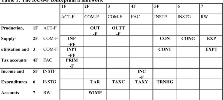
Table 1: The SAM-F conceptual framework

1F 2F 3 4F 5F 6 7

ACT-F COM-F COM-F FAC INSTP INSTG RW

Production, 1F ACT-F OUT

-F

OUTT -F

Supply- 2F COM-F INP

-FF

CON CONG EXP

utilisation and 3 COM-F INPT

-FF

CONT EXPT

Tax accounts 4F FAC PRIM

-F

Income and 5F INSTP INC

-F

Expenditures 6 INSTG TAR TAXC TAXY TRNHG

Accounts 7 RW WIMP

Corresponding to how a VAT is represented the standard model the matrix of taxes on household consumption CONT>0 and the matrices of taxes on outputs OUTT-F, taxes on intermediate consumption, INPT-FF, export taxes, EXPT, andtariffs TAR areall 0.

7

By theorems of tax equivalence, we may alternatively define a VAT by assuming that domestic production and imports are taxed at the same rate and reimbursed on intermediate consumption in the formal sector and exports.

However, alternatively and in closer correspondence with administrative practice a VAT may be represented by CONT=0, but instead OUTT-F>0, INPT-FF<0, EXPT<0, and TAR>0. This representation is more relevant for the assessment of the administrative costs associated with a VAT compared to other tax structures, for example taxes on output. It suggests 1) that a VAT will be associated by considerable higher administrative costs than a system of output taxes OUTT-F as it does not require the monitoring of intermediate inputs and foreign trade and the well-known problems associated with VAT fraught, and 2) that a that the additional administrative costs of supplementing a VAT with additional tariffs payments would be limited as the VAT requires the monitoring of imports. For the discussion of whether border taxes are desirable, the first representation is preferable to avoid confusion between tariffs and withholding taxes on imports, but for the comparison of the administrative costs associated with VAT with those of other tax structures, the second representation is preferable.

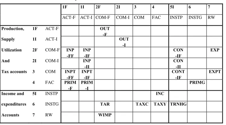
The SAM for the model with representation of informal sector production, the DUAL SAM, is provided in Table 2. It is obtained from SAM-F by splitting the household income expenditure account, 5F, into two accounts, a production account for informal sector production 1I and a redefined household income expenditure account 5I, by adding a supply-utilisation account for commodities produced in the informal sector, 2I. In the DUAL SAM with a VAT, INPT-FF, EXPT, and TAR are 0, as in the SAM-F, whereas the tax on intermediate consumption for the production of informal sector goods, INPT-IF, is different from zero; in fact corresponding to the same rates of VAT as those applied on the household’s final consumption of goods produced in the formal sector, CONT-IF. By construction we have that the household purchases of goods produced in the formal economy, CONT = CONT-IF + INPT-FF.

Table 2. The DUAL SAM conceptual framework

1F 1I 2F 2I 3 4 5I 6 7

ACT-F ACT-I COM-F COM-I COM FAC INSTP INSTG RW

Production, 1F ACT-F OUT

-F

Supply 1I ACT-I OUT

-I

Utilization 2F COM-F INP

-FF INP -IF CON -IF EXP

And 2I COM-I INP

-II

CON

-II

Tax accounts 3 COM INPT

-FF INPT -IF CONT -IF EXPT 4 FAC PRIM -F PRIM -I PRIMG

Income and 5I INSTP INC

expenditures 6 INSTG TAR TAXC TAXY TRNHG

4. Application of general insights from Public Economics

In this section, we address from a theoretical point of view the question of whether border taxes are desirable in an economy with informal sector production when government revenue is raised by a VAT. This is the same question which Keen (2008) considers. Our analysis confirms his conclusion that when taxation is not associated with administrative costs, production efficiency is desirable whatever the size of the informal sector and whether or not informal sector production is associated with (untaxed) profit. However, we deepen the insight provided by Keen’s analysis in two ways, 1) by providing a simple proof under more general assumptions, based on a general equilibrium rather than a partial equilibrium model, and 2) by reaching this result with reference to standard theorems of public economics rather than deriving the results from first principles. This illustrates the benefits of embedding the informal sector production in the household utility function, as it facilitates interpretation and derivation of results, a point made by Atkinson and Stern (1980) in relation to the seminal paper of Becker (1965) on a theory for the allocation of time. We also on this basis exploit other theoretical results from Public Economics to gain insight into what determines the optimal tax system in an economy with a large informal sector where taxation is associated with administrative costs.

4.1 The Diamond and Mirrlees (1971) production efficiency theorem

The Diamond and Mirrlees (1971) Production Efficiency Theorem says that in an economy without untaxed profit, although lump-sum taxation is not feasible, optimal taxation still requires production efficiency when all market transactions can be taxed at their optimal level at no costs. We have assumed that production in the formal sector takes place under constant returns to scale and therefore is associated with no profit. It therefore follows directly from this theorem that if taxation is not associated with administrative costs, then production efficiency and thus free trade is desirable in the economy represented by the general equilibrium conditions (1)-(13). Under the assumption that taxation is associated with no administrative costs, in the general model (1)-(13), the optimal tax system therefore involves only taxation of household net demand, t



t t ,t t₀, _{1 2}, ₃



and no taxation of intermediate inputs or border transactions, i.e. ti 0, 1, 2, 3i and tW 0, i.e. a VAT and no border taxes. However, the optimal VAT in general requires the rates of VAT to be differentiated between commodities.

The question is now if this answer carries over to the model with informal sector production. The received wisdom is that for the Production Efficiency Theorem to be valid, the household must receive no untaxed profit. A question of particular interest is therefore if VAT without border taxes is also desirable in the case of (untaxed) profit in the informal sector.

The conditions for an optimal choice of x_i, 0,1, 2, 3i and c₀i, 1, 2, 3i are represented by (24)-(30), whereas the conditions for the optimal choice of x_i, 0,1, 2, 3i , without indication of how the household uses its consumption of the primary factor c₀within the household, are represented by

(6)-(8). The model represented by the general equilibrium conditions (1) to (5), (9)-(13), and (24)-(30) is therefore a special case of the general model represented by the general equilibrium conditions (1)-(13) . Because a VAT without border taxes is the optimal solution in the general model, it is therefore also the optimal solution in the more specific model, even if production in the informal sector is associated with untaxed profit.

Given that it has not been generally recognised in the literature that production efficiency in the formal sector is not compromised by informal sector production being associated with untaxed profit, it is worthwhile to pause to provide an intuitive explanation of this result.

In fact, contrary to the received wisdom; if all commodities can be taxed at no costs, production efficiency is desirable also in the case of untaxed profit in the formal sector. When the government’s requirement exceeds the value of the profits at producer prices, then the optimal tax system involves the value of the profits to the household being wiped out by the level of consumer prices being set infinitely high relative to the level of producer prices while not imposing sector specific producer taxes



0,1 2 3



i i i i i t t ,t ,t 

t , i=1,2,3, i.e. by maintaining production efficiency (cf. Munk 1978, Munk 1980). It is therefore not possible as in Dasgupta and Stiglitz (1971) and in number of subsequent contributions (for example Boadway and Sato 2009) in a model with untaxed profit in the formal sector to assume the primary factor as untaxed as a matter of normalisation without loss of generality. One may naturally assume that for some reason the primary factor cannot be taxed, but this then begs the question of what is the supporting empirical evidence for such an assumption8.

However, the analysis of the optimal tax system subject to the restriction that market transactions in the primary factor cannot be taxed, as in Dasgupta and Stiglitz 1971 and Munk 1980, provides insight into why production efficiency is not desirable in the presence of untaxed formal sector profit, but desirable in the presence of untaxed informal sector profit. When the government due to this tax restriction cannot raise the required tax revenue by a proportional tax system (taxing market transactions in produced commodities and subsidizing the market supply of the primary factor) effectively taxing formal sector profit, the social value of a unit of income to the government is larger than to the household. Increasing producer taxes, ti 



0,t ,t ,t₁i ₂i ₃i



, i 1, 2,3 makes it possible to manipulate producer prices reducing the household’s profit income and increasing the government’s tax revenue. To do so is desirable to the point where the marginal benefit in terms of social welfare of this “transfer” is equal to the marginal cost due to the distortion of production.

In contrast, in the case of untaxed informal sector profit, there is no such trade-off, because the

informal sector profits



₀



1,2,3 , , i i i i q q Q 

 



 depend on consumer prices. Taxes applied to formal sector transactions therefore have no effect on informal sector decisions, as these depend only on consumer prices which the government by assumption can set independently of producer prices at no costs.

With no formal sector profit, the equations for the model with informal sector production are therefore homogenous of degree zero in consumer prices, also in the presence of informal sector profit. As we

8

The fact that the optimal solution based on a model with untaxed profit involves infinite tax rates is an indication, which has largely been ignored in the literature, that it is highly problematic to provide tax advice based on a model which does not represent the administrative costs of taxation.

have assumed that production in the formal sector takes place subject to constant returns to scale, we can therefore as a matter of normalisation without loss of generality assume the market transactions of one commodity, for example the primary factor, are not taxed, even if informal sector production is subject to decreasing returns to scale.

4.2 The Corlett and Hague (1953) insight

The Corlett and Hague (1953) analysis of optimal taxation suggests that those commodities most complementary with leisure should be taxed at the highest rates. We use this result to gain insight into how certain characteristics of the informal sector influence the optimal tax system.

The matrix of compensated demand-supply elasticities

In the case where production in the informal sector takes place under constant returns to scale, i.e. where



₀i,



i i

C c x , i1,2,3, are homogenous of degree 1, and where household preferences may be represented by a utility function U c C C C C



₀0,



₁, ₂, ₃





, where C C C C



₁, ₂, ₃



is also homogenous of degree 1, and where U c C



₀0,



is a utility function with standard properties, we define









0 0 0 0 0 , , Min s.t. , / i i i i i i i i i i i i c x Q Q q q  q c q x C c x  C   , iC









1 2 3 1 2 3 1 2 3 , , _{i 1,2,3} , , Min Q_{i i} s.t. , , / C C C Q Q Q Q Q C C C C C C     _{  } 









0





0 0 0 0 0 0 0 , , , Min s.t. , c C M q Q u _ q c QC U c C _   

Incorporating household production in the utility function yields



 

 









0 1 2 3



0, 1 1, 0 , 2 2, 0 , 3 3, 0

uU c C C x c C x c C x c (31)

and the corresponding expenditure function becomes



 

 









0, 1 0, 1 , 2 0, 2 , 3 0, 3 ,



M q Q Q q q Q q q Q q q u

M   (32)

By the derivative property of expenditure functions and the definition



q q q q u0, 1, 2 3,



M q Q Q q q



0,



1



0, 1

 

,Q2 q q0, 2

 

,Q q q3 0, 3





,u



M   (33)

by differentiating (33) we express the demand system x_i

 

q,u , 0,1, 2, 3i in terms of properties the expenditure function which explicitly represents informal sector production

 

0 0 1,2,3 0 0 , j j j Q M M Q x u q Q  Q q          



  q   (34)

 

, i i i i Q M Q x u Q Q q        q  i1,2,3 (35) where ₀0 0 M c q     , M C Q  _   , j j C Q Q C    and 0 0 j j j Q c q C    .

Defining 1 0 0 0 i i i i q c a Q C

 as the share of the costs of the consumption of the primary factorin the total costs of composite i, and 2 j j

j

Q C b

QC

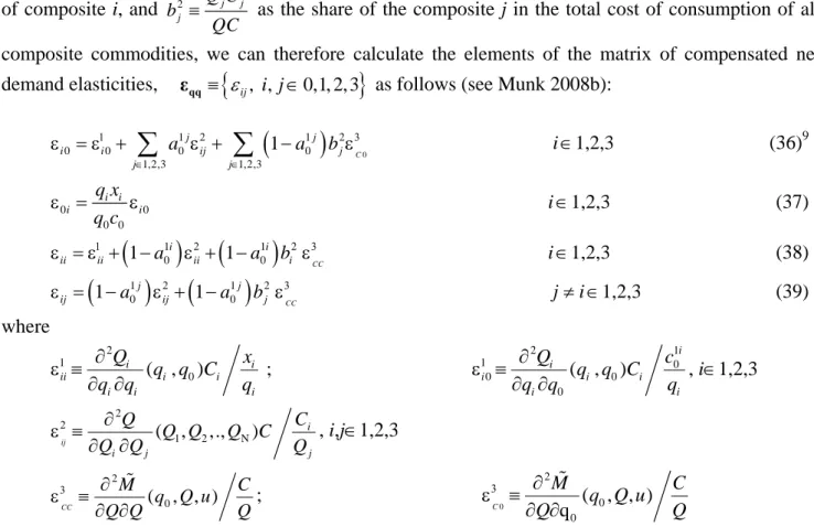
 as the share of the composite j in the total cost of consumption of all composite commodities, we can therefore calculate the elements of the matrix of compensated net demand elasticities, εqq 



_ij, ,i j0,1, 2, 3



as follows (see Munk 2008b):





0 1 1 2 0 0 0 0 1,2,3 1,2,3 1 C j j i i ij j j j a a b         



 



  1,2,3i (36)9 0 0 0 0 i i i i q x q c    i1,2,3 (37)



1

 

1



2 0 0 1 1 CC i i ii ii a ii a bi             i1,2,3 (38)



1





1



2 0 0 1 1 CC j j ij a ij a bj          1,2,3j i (39) where 2 1 0 ( , ) i i ii i i i i i Q x q q C q q q      ; 2 1 1 0 0 0 0 ( , ) i i i i i i i Q c q q C q q q      , i1,2,3 2 1 2 N ( , ,., ) ij i i j j C Q Q Q Q C Q Q Q       , i,j1,2,3 2 0 ( , , ) CC M C q Q u Q Q Q        ; 0 2 0 0 ( , , ) q C M C q Q u Q Q       

The Corlett and Hague (1953) conjecture says that commodities which a complementary to the use of the primary factor in the household sector (complementary with leisure), i.e. with small _i0, should be taxed at a relatively high rate (see Munk 2010 why in the case of more than two produced commodities this result should be considered as a conjecture rather than a theorem).

The CES-UT parameterisation

The CES-UT utility function is defined as (see Munk 1998, Annex 1)



 

 









0 1 11 2 12 2 13 2 3



0, 1 1, 0; , 2 2, 0; , 3 3, 0; ; U c C C x c  C x c  C x c    (40) where 1 ; 0 ( , i i) i i C x c  , iC,



2



1, 2, 3; C C C C  and



0 3



0 , ;

U C c  are CES functions characterised by elasticities of substitution 1i

, iC, 2

and 3

, respectively. The structure of the CES-UT is illustrated in Figure 1.

Figure 1: The structure of the CES-UT utility function

u 3

9

This formula may alternatively be derived from using that ₀

C i ij j     



and 1 1 0 i ii    and 0 3 3 C CC    .

C c₀0 2  1 C C₂ C₃ 11  12 13 1 x c10 x2 2 0 c x₃ c30

In the case of the CES-UT,     _ii _i0 a1₀i1i,  _ij b_j2 for 1,2,3i, j i





2

1 ii bi       for 1, 2, 3i and 0 (1 ) CC C c          , where ₀ 0 0 QC c q c QC   , we have











1 1 1 2 1 0 1 0 1 1 0 (1 ) i i i i ii a  a bi  a bi c            1, 2,3i (41)



1



2



1



0 0 1 j 1 j (1 ) ij a bj a bj c         i j, 1, 2,3 (42)





1 1 1 2 0 0 1 0 (1 ) i i i i a  a a  a c          1, 2,3i (43)







1 1 1 2



0 0 0 0 0 1 (1 ) i i i i i i q x a a a a c q c            1, 2,3i (44) where



1₀



1,2,3 1 i _j j a a b  



 .

Representing the Corlett and Hague (1953) insight in applied work is a challenge. On the one hand optimal tax systems cannot be calculated based on demand systems estimated based on flexible forms because globally they do not satisfy the assumptions of quasi-concavity and monotonicity, on the other hand functional forms widely used in other applied work, which satisfy these assumptions, such as those belonging to the CES family, impose separability between consumption and leisure restricting the optimal solution to be a proportional tax system. Furthermore data on informal sector production are in general derived from quite different sources than on market transactions. The CES-UT makes it possible to address this challenge. It makes it possible to estimate the 1i, 1, 2, 3i , based on survey data from observations of informal sector production in terms of C x c_i , _i, ₀i, and then to estimate the 2

and 3 parameters based on time series of market transactions of x i_i, 0,1, 2, 3 and market prices , 0,1, 2, 3

i

p i , imposing the estimated values of 1i, 1, 2, 3i and the elasticity formulae (41)-(44).

How the optimal tax system depends on informal sector characteristics

In the special case where only the consumption of commodity 1 requires the use of the primary factor (see Figure 2), a  



1 a11₀



b₁, we have













11 11 11 2 11

10 a0 1 a0 1 b1  1 a0 b1(1 c)



        1, 2,3i (45)

The interpretation of this equation is that if

 the household consumption of commodity 1 x₁ requires a large amount to the primary factor (i.e. if a1₀iis large)

 the (intermediate) consumption of commodity 1 and of the primary factor c1₀ in the production of the informal commodity C₁ , are complementary, i.e. if 11 is small relative to 2

 the consumption of informal sector commodity C₁ is a close substitute to the household consumption of x₂, x₃, i.e. if 2is large relative to 11,

then the optimal tax rate on the household’s purchases of commodity 1 will be relatively high.

4.3 The Stiglitz and Dasgupta (1971) insight

From the outset Stiglitz and Dasgupta (1971) pointed out that the Diamond and Mirrlees (1971) Production Efficiency Theorem rests on the rather unrealistic assumption that all market transactions can be taxed at their optimal level at no costs. When this assumption is not satisfied, production efficiency and free trade may not be desirable, an implication of particular importance in developing countries, in general characterised by weak administrative infrastructure making tax collection particularly difficult. It is in fact generally recognised that for the design of optimal tax systems administrative costs are important10

It is also widely accepted in the literature, that a progressive income tax combined with a VAT at a uniform rate without the use of border taxes is the best system of taxation in developed countries. This position has found its justification mainly based on two arguments. First, that with a progressive income tax, the scope for increasing social welfare by a differentiated rather than a proportional system of commodity taxation is small compared with the administrative costs involved; and second, that the use of border taxes will introduce production inefficiency. The first argument is often justified with reference to Atkinson and Stiglitz (1976), who in a simplified model show that there is no need for differentiated commodity taxation with a pre-existing optimal income tax. The second argument refers to the Diamond and Mirrlees (1971) Production Efficiency Theorem, mentioned above.

However, there is also a consensus in the profession supported by research by the IMF and the World Bank that in developing countries raising tax revenue by income taxation is de facto impossible due to the associated high administrative costs. As emphasised by Emran and Stiglitz (2007), and also recognised in Ebrill et al (2001, p71), the fact that developing countries cannot raise a significant amount of tax revenue by income taxation, means that the insight by Atkinson and Stiglitz (1976) cannot be used to provide a rationale for the application in developing countries of a VAT at a uniform rate.

10

E.g. Ebrill et al. (2001) in the Preface at p xii, p75 and in Chapter 16 stress the importance of taking administrative concerns into account. Although they do not explicitly represent such costs in their model, Emran and Stiglitz (2005) also put great emphasis on the importance of administrative costs for tax design in developing countries.

Furthermore, when the VAT is constrained to be at a uniform rate, it is not possible to justify free trade with reference to the Diamond-Mirrlees (1971) Production Efficiency Theorem. In developing countries with a large informal sector, a VAT at a uniform rate imposes a considerable distortion of the labour supply by encouraging the use of labour in the informal sector. There are therefore large potential benefits to be obtained from a differentiated VAT which encourages the supply of labour to the formal sector. When a differentiated VAT is not possible due to the administrative costs involved, the use of border taxes to obtain the same objective may be desirable, as suggested by Stiglitz (2003). As Emran and Stiglitz (2005) have pointed out, the size of the formal sector in this case plays an important role for whether the use of border taxes is desirable or not (see also Munk 2008a).

The IMF and World Bank recommendations with respect to taxation in developing countries to abolish border taxes and to implement a VAT at a uniform rate11 may therefore be seen as the application to developing countries of what is widely considered a reasonable system of commodity taxation for developed countries, but neglecting the important differences between developed and less developed countries, in particular with respect to administrative costs of taxation and the relative size of the informal sector.

4.4 The challenge

It is one thing theoretically to establish that administrative costs may justify diversions from free trade; it is another matter whether such costs do in fact justify the use of border taxes. The data required to specify a general equilibrium model to represent the economy of a developing country, are in general not readily available, and in particular, there is still little empirical evidence on the administrative costs associated with different tax systems and on production in the informal sector. For a given developing country at a given point of time, whether free trade is desirable or not therefore remains an open question until the necessary empirical evidence has become available and applied. However, in order to contribute to eventually to make it possible to provide a definite answer to the question, we present a quantitative example involving the use of a stylized Computable General Equilibrium (CGE) model with explicit representation of the informal sector. By constructing this stylized CGE model representing a prototype developing country, we put numbers to the theory with the objective to get a better idea of the potential importance of administrative costs of taxation and of the size and production technology in the informal sector for the choice of an optimal tax-tariff system. It also serves to provide guidance on how to gather the relevant data and to use such data to estimate the relevant model parameters.

5. Specification of empirical model

In this section, we formulate a parameterised model of a prototype developing country. However, we first simplify the theoretical model specified in Section 2 to facilitate comparison with the partial equilibrium model used by Keen (2008) (see Annex 1).

11

In fact, the World Bank and the IMF for distributional reasons recommend zero rating for basic food stuff and taxation of certain luxury articles in addition to a uniform VAT. However, although highly relevant we do not in the context of this article consider the distributional aspects of taxation.

We assume that the formal part of the economy involves transactions in three produced commodities: Manufactured good (1), Cash crop (2) and Food(F) (3), all goods traded both domestically and internationally. At world market prices, the economy is competitive only in the production of Food(F), which we therefore assume to be the export good12. Furthermore, we assume that the Manufactured good (1) is used as intermediate input in the production of Food(F), and as such not subject to taxation and as intermediate input in the production of Food(I) where in contrast it is taxed. As a matter of normalisation we assume that t₀ 0 and t₃W 0.

The general equilibrium conditions to be satisfied by a tax system



, 1,2,3, , 1, 2W



i i

t i t i

  

τ now

become (compare with (1) to (5), (9)-(13), and (24)-(30)): Conditions for profit maximisation





3 3 0, 1 p c p p (46)





3 1 0 1 3 1 , c v p p , y p    (47)

Conditions for utility maximisation



0, ,1 2, 1,



M q q q Q u = 1





0 0 1 1 0, 1, 1 q Q C G q q C (48)





1 1 1 C 0, 1, 1 Q G q q C (49)





0 0 0 0, 1, 2, 1, c M q q q Q u (50)





1 1 0, 1, 2, 1, C M q q q Q u (51)





1 1 0 0 0, 1, 1 c G q q C (52)





1 1 1 0, 1, 1 x G q q C (53)



0, 1, 2, 1,



i i x M q q q Q u i2, 3 (54) 0 1 0 0 0 0 x c c  (55) Material balance 0 v₀ x₀ x₀G (56) 1 1 1 W y  v x (57) 2 2 W y  x (58) 3 3 3 W y  y  x (59)

Balance of trade constraint

i 1,2,3 W W i i p y 



=0 (60)

Government's budget constraint

0 0 i=1,2,3 i=1,2 0 W W G i i i i t x  t y  p x 





(61) 12

There will in general be values of taxes where this is not the case (see Munk 2008a). However, for the sake of ease of exposition we ignore this possibility.

We represent the formal sector production technology for Food(F) by a CES unit cost function





3 3 1 , ; 0 c p p s , where 3

s is the elasticity of substitution between inputs of the primary factor, Labour, and of inputs of the Manufactured good.

The household’s preferences with respect to Pure leisure c₀0 and the household’s produced commodities C C C₁, ₂, ₃ we represent by U c C C C C



₀0,



₁, ₂, ₃; 2



; 3



where



2



1, 2, 3;

C C C C  and



0 3



0, ;

U c C  are homogenous CES functions characterised by elasticities of substitution 2

and 3

, respectively (see Section 4.2).

The household uses its purchases of the Manufactured good to produce Food(I) according to a constant returns to scale CES production function



1 11



1 1 0, 1;

C C c x  , where 11

is the elasticity of substitution between Labour and the Manufactured good, and Q q q₁



₀, ₁;11



the corresponding unit cost function. For the two other informal sector goods, C₂ x₂ and C₃ x₃.

Incorporating the household production functions in the utility function we obtain the CES-UT utility

function,



0





1 11



2



3



0, 1 1, 0; , 2, 3; ;

U c C C x c  x x   illustrated in Figure 2.

Figure 2: The structure of household preferences imbedding the informal sector production

u

3



C: Aggregate consumption c₀0: Pure leisure

2



1

CFood (I) x₂: Cash crop x₃ : Food(F)

1 1  1 x: Manufactured 1 0 c

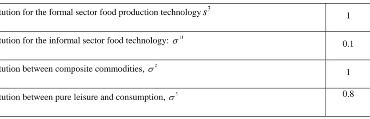
Elasticity of substitution for the formal sector food production technologys3 ₁ Elasticity of substitution for the informal sector food technology: 11

0.1 Elasticity of substitution between composite commodities, 2 ₁ Elasticity of substitution between pure leisure and consumption, 3 0.8

We derive the benchmark data set from the DUAL SAM (see Annex 2)13 where the informal and the formal production of food, Food(F) and Food(I), are represented by separate activities with different cost structures. The DUAL SAM has been constructed so that the share of National Income (NI) is high, 52% 14, representative of the large share of the labour force being employed in the informal sector in many developing countries.

It is now possible using the elasticity formulae (41)-(44) based on benchmark data set and the values of substitution elasticities 11, 2 and 3, specified in Table 3, to calculate the matrix of compensated net demand elasticities εqq 



ij, ,i j0,1, 2, 3



. These are provided in Table 4. Notice,

that the compensated elasticities of demand with respect to the price of the untaxed use of the primary factor in the household sector for the Manufactured good at 0.131 is smaller than for Cash crop and Food(F), both equal to 0.806. Based on the Corlett and Hague insight we therefore expect the optimal tax rate on the Manufactured good to be higher than on Cash crop and Food(F).

Table 4: Consolidated compensated demand and supply price elasticities

ij



Manufacturing Cash crop Food (F) Labour

Manufacturing -0.239 0.032 0.075 0.131 Cash crop 0.086 -0.968 0.075 0.806 Food (F) 0.086 0.032 -0.925 0.806 Labour -0.046 -0.105 -0.245 0.396

Note: The elasticities have been calculated based on the substitution elasticities specified in Table 3 and the benchmark data on informal sector production and household consumption derived from the DUAL SAM provided in Annex 2 Table 4.

6. Simulation results

We assume that the government considers four different tax structures:

1

 : Only VAT at uniform rate,

2

 : No restrictions on the set of feasible tax instruments,

3

 : VAT at uniform rate and border taxes, and

13

This CGE model is similar to that in Piggott and Whalley (2001) except that they do not incorporate informal sector production in the utility function.

14

The value added in formal and informal production is 23 and 30.5, respectively, and the value of the Government’s consumption of the primary factor of 5. The share of informal production in National Income is thus 0.52=30.5/(30.5+23+5).

4

 : Only border taxes.

We make no assumptions about the administrative costs associated with each tax structure,

 

, 1, 2, 3, 4

B j j , as there is little empirical evidence on which to base such assumptions, but we expect on theoretical grounds thatB

 

2 B

 

3 B

 

1 and B

 

2 B

 

4 (see Munk 2008a).

Disregarding administrative costs of taxation, the optimal tax systems for the different tax structuresj, 1, 2, 3, 4j , are provided in Table 5.

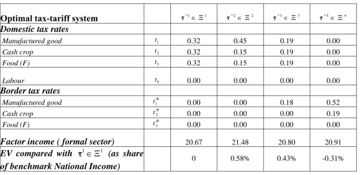
Table 5: Optimal tax-tariff systems and administrative costs

Optimal tax-tariff system _τ* 1 1 _τ* 2 2 _τ* 3 3 _τ* 4 4

Domestic tax rates

Manufactured good t1 0.32 0.45 0.19 0.00

Cash crop t2 0.32 0.15 0.19 0.00

Food (F) t3 0.32 0.15 0.19 0.00

Labour t0 0.00 0.00 0.00 0.00

Border tax rates

Manufactured good 1 W t _{0.00 0.00 0.18 0.52} Cash crop 2 W t _{0.00 0.00 0.00 0.19} Food (F) 3 W t _{0.00 0.00 0.00 0.00}

Factor income ( formal sector) 20.67 21.48 20.80 20.91

EV compared with _τ1 1

(as share of benchmark National Income)

0 0.58% 0.43% -0.31%

For 1, where the government’s expenditures must be financed by a VAT at a uniform rate, this rate is 32%. This tax system serves as benchmark for the comparisons of the social welfare achievable under the alternative tax-tariff structures.

For 2, there are no restrictions on the government’s use of commodity tax instruments. The optimal tax system involves production efficiency and hence W

=0

t . The optimal differentiation of commodity tax rates represents a trade-off between the objective of encouraging the supply of labour to the formal sector, and the objective of not distorting the consumer prices of produced commodities (see Munk 2010). As the Manufactured good is complementary with the large (untaxed) use of the primary factor in the informal sector, the optimal tax on the consumption of the Manufactured good is at the relatively high rate of 45%, whereas the consumption of Cash crop and Food(F) is taxed at only 15%.

For 3

, where the government’s revenue requirement can be financed by a VAT at a uniform rate supplemented by border taxes, production efficiency is not desirable. The optimal tax system now involves a three way trade-off between the same two objectives as in the case of 2, and in addition the objective of limiting the distortion of the input price of the Manufactured good in the production of Food(F). The optimal solution involves a VAT at a uniform rate of 19% supplemented by a tariff on the imports of the Manufactured good of 18%; representing a price wedge between the consumer price and the world market prices of 40%15. Due to the objective of limiting the distortion of the use of inputs in the production of Food(F), this rate is lower than for _τ*2 2

where the optimal VAT rate for the Manufactured good is 45%.

Finally, for 4, where the government’s revenue requirement can be financed only by border taxes, the optimal solution involves differentiation of tariff rates motivated by three objectives (cf. Munk 2008a):

The two objectives which determine the optimal tax system in a closed economy

15

- to encourage the supply of labour to the formal sector ( Objective 1), and - not to distort the consumer prices of produced commodities (Objective 2) and in addition third objective,

- to encourage the export of Food(F) (Objective 3)16 Objective 2 draws, as in the case of 3

, in the direction of a relatively high tariff on the imports of Manufactured good. Objective 3 suggests, on the one hand, that it is desirable to strive for a relatively high tariff on the imports of Manufactured good which in household consumption to discourage the consumption of Food(F), the export good, but, on the other hand, a relatively low tariff on the Manufactured good to limit the distortion in the production of Food(F). With the current parameterisation the Manufactured good and Food(F) are equally complementary with the consumption of Food(F) with ₁₃ ₂₃ 0.075 (see Table 4)17. Objective 2 of encouraging the supply of labour to the market dominates Objective 3 of encouraging the exports of Food(F) with the result that the optimal tariff on the imports of the Manufactured good at 52% is considerably higher than the tariff on Cash crop at 19%.

The optimal tax systems for the different tax structures j, j1, 2, 3, 4, provided in Table 5, leave open the question of what is the overall optimal tax system when administrative costs are taking into account. To give an idea of the size of administrative costs required to justify the use of border taxes to supplement or replace a VAT at uniform rate, we calculate the change in administrative costs required to make the optimal tax systems under the tax structures _3

and _4

, respectively, equivalent in welfare terms to _τ1_{. These results are reported in Table 6.}18 _{The results show that border taxes are desirable as}

an alternative or as a supplement to a VAT system, if either 1) the administrative costs associated with

3

 is at most 0.29% of NI higher, or 2) those associated with _4

at least 0.35% of NI lower, than those associated with 1

.

Table 6: Administrative costs making _τ*i ~_τ*1

Optimal tax-tariff system τ*3 3 τ*4 4

Required saving of administrative costs as share of National Income 0.29% -0.35%

The cost of financing the government’s revenue requirement by border taxes rather than domestic taxes increases progressively with the government’s revenue requirements. If for example the government’s requirement increases from 5 units of labour (as has been assumed in calculating the results reported above) to 10 units, the saving in administrative costs needed to finance the government’s revenue requirement solely by border taxes rather than by a VAT at a uniform rate increases more than threefold from 0.35% to 1.15% of NI.19 As the share of the government budget in

16

For border taxes to raise revenue to the government the tax system *4

τ must discouraged the exports of Food (Formal sector). Objective 3 does not apply in the case of 3 since under this tax structure the justification for the use of border taxes is not to raise government revenue directly, but to encourage the supply of labour to the market.

17

However, this is an artefact of the parameterisation of the model. The CGE model may easily be modified to represent that a relative low tariff on the Manufactured good will be desirable to encourage the production, and thus the export of

Food(F).

18

The figures differ from the EVs reported in Table 6, as they have been calculated taking the administrative costs of taxation into account.

19

Just with reference to the increasing size of the government’s share of consumption in NI, Kimbrough and Gardner (1992) explain why the importance of tariff revenue in the US has diminished over time. Our analysis confirms this insight