Neural Program Lattices

(1)

Neural Program Lattices

Learning through Weak Supervision

James D. Rampersad

Department of Engineering

University of Cambridge

This dissertation is submitted for the degree of

MPhil in Machine Learning,

Speech and Language Technology

(2)

(3)

Declaration

I, James David Rampersad of St Edmund’s College, being a candidate for the M.Phil in Machine Learning, Speech and Language Technology, hereby declare that this report and the work described in it are my own work, unaided except as may be specified below, and that the report does not contain material that has already been used to any substantial extent for a comparable purpose. Total word count: 7483

Signed:

James D. Rampersad August 2017

(4)

(5)

Acknowledgements

I would firstly like to thank my two supervisors for their help throughout the research and write-up of this thesis: Professor Bill Byrne of Cambridge University and Dr Nate Kushman of Microsoft Research. I’d also like to acknowledge more generally the excellent teaching I’ve experienced throughout the course of my studies this year at the Cambridge University Engineering Department.

(6)

(7)

Abstract

Learning useful abstractions from superficially complex data has been a long-standing problem in Machine Learning. TheNeural Program Lattice[7] is an important step forwards, but still requires a few hand-crafted abstractions to facilitate learning. In this thesis we investigate the possibility of removing the remaining supervision entirely, enabling inference of latent functional hierarchies from purely elementary operations.

Our preliminary work highlights an aspect of the existing objective function that prevents learning in the absence of at least some strong supervision and we devise a new, marginal loss that facilitates training when provided with only weak supervision.

While learning can occur under this new loss, we show that the model acts essentially as a sequence to sequence learner, failing to exploit the advantages of the program hierarchy. We attribute this to the presence of a set of a dominant local minima in weight space and devise a new environment,

Bitflipto deduce whether certain incentives can facilitate basic functional inference. Our results indicate that the NPL struggles to encapsulate behaviour without pathological constraints. We conclude with a discussion as to possible reformulations of the NPL framework to more naturally approach the inference problem.

(8)

(9)

List of figures

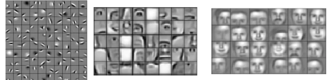
1.1 A simple sequential hierarchy, the lowest level discrete sequence can be effi-ciently represented by two levels of abstraction. Once the hierarchy is learnt, reasoning/prediction at the top level reduces complexity by a factor of 6. . . 1 1.2 Features learnt by convolutional filters in a facial recognition task. Image by

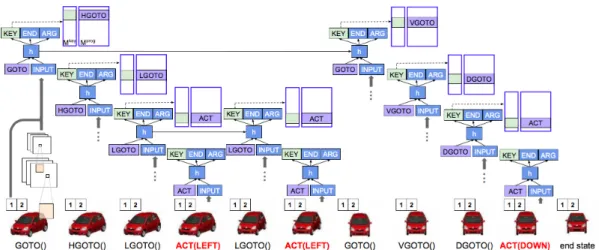
Honglak Lee and colleagues (2011) as published in “Unsupervised Learning of Hierarchical Representations with Convolutional Deep Belief Networks”. . . 3 2.1 An example of one algorithmic task from Neural Programmer-Interpreters (2016)

Reed and De Freitas. The controller is given a desired angle and elevation and must control the camera’s azimuthal angle and height so as to achieve the correct viewpoint. In the execution trace above, GOTO,HGOTOand LGOTOare functions

while ACT is the name given to elementary operations that change the world-state (the visual representation of the car). Each of theseACTcalls also contain

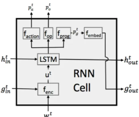
arguments, that specify the angle to turn or height to rise. . . 6 2.2 The LSTM controller, shown in context with environmental encoders f_enc and

actuators f_action, f_op, f_prog. The input and output program embeddings are labelled

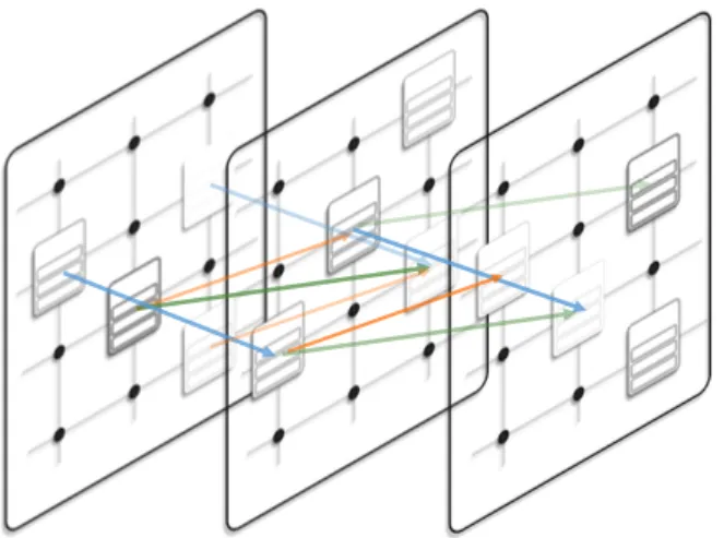
gt_inandgt_out respectively. (This image is from Neural Program Lattices [7]) . . . . 7 2.3 The lattice of execution paths. Each point in the grid represents a grouping by

elementary operationiand call depthl. The recursive variableyt_i,l is computed across all these nodes sequentially, denoting the probability that at a timet the controller has correctly calledielementary operations and exists at a depthl. This image is taken from [7] . . . 9 3.1 The weight-space problem, characterised by strongly attractive local minima that

(12)

xii List of figures

3.2 A time-merged plot ofyt_i,l probability flow through the lattice under fully super-vised pre-training and the original loss function after 10,000 iterations. Colour intensity corresponds to higher values ofyt_i,l (summed acrosst). Training appears to have converged as there is only a single path, that successfully encapsulates all its actions within functions -shown by the majority of calls originating from the second level of the hierarchy. The pathPOPs to the top level before calling a new function withPUSH, returning to the second level. This is the behaviour we would hope to see inferred in the absence of strong supervision. This example is taken from theNanocraftdomain. . . 13 3.3 Probability flow through the lattice under the original loss function in the

ab-sence of strong supervision. Note there is no horizontal flow ofyat all, with all probability mass lost through incorrect action calls orPOPPINGtoo soon. . . 13 3.4 The time-merged lattice under the new, marginal loss function. Probability now

propagates throughout the whole of the lattice, with latent paths making a function call at approximately the point where the nature of the task changes significantly (as will be seen in Section 3.3). This was not observed however during the greedy-decoding runs.. . . 14 3.5 The time-merged lattice under the marginal sub-sequence loss. Probability flows

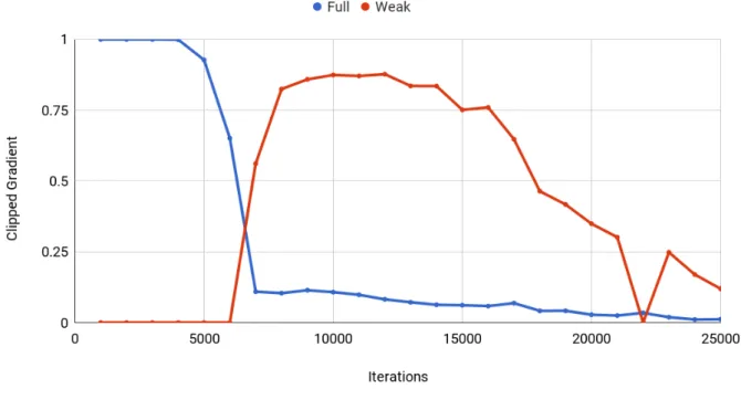
throughout the lattice, with a portion of the latent paths calling functions and moving into the second level of the hierarchy. In greedy decoding, the controller LSTM calls only functions of a single action in length, corresponding to placing a block in theNanocraft domain. As will be discussed in Section 3.3. . . 15 3.6 a) The evolution of clipped gradient during a training run in which fully supervised

samples were present. Red corresponds to the average gradient of weakly super-vised samplesunder the original loss function. Blue shows the mean gradient of the strongly supervised samples (trained with the loss function from NPI [9]). Note that gradient for the weak samples is zero at first before rising steadily as more probability mass reaches the terminal node due to the guidance from full supervision. b) The clipped gradient across three runs using entirely weak super-visionwith the new marginal loss function. Note that there is now a workable gradient immediately which slowly decreases as the model fits to the training data. 16 3.7 TheNanocrafttask. The agent receives input from from three locations, the grid

world embedding (from a convolutional encoder), a natural language embedding (specifying the type of house, size and location to build) and an embedding from the currently running program. Some blocks of the house are already placed in the grid. The agent must avoid placing blocks twice in the same location so needs to monitor the world state at all times. . . 17

(13)

List of figures xiii

3.8 The mean training curves, for 16, 32, 64, 128 and 512 weakly supervised samples. As indicated by the standard-deviation, training is highly volatile under gradient descent. There is a general trend that loss decreases most rapidly for those with the fewest numbers of samples as the network can rapidly adapt its parameters to fit the sequences. A minimum of two trials are performed in each case, with 512 and 128 repeated in greater number due to higher variation in results. Training loss here is the negative log-probability of calling the correct elementary operations independently and then callingPOPto terminate the algorithm. . . 18 3.9 The individual training runs performed with 512 weakly supervised samples. Note

the fact that curves tend to follow one of three tracks possibly a result of different valleys in weight space. . . 19 3.10 The training runs for the model with 16 Samples. Note that only one sample

appears to fully explain the training data. . . 19 3.11 The average progression of models trained under each number of samples through

the Nanocraft program. There is a clear trend for the progression to increase with the number of samples, as one would expect. The anomalous result for 128 samples reflects the volatility of the training process, with none of the performed trials completely fitting to the training samples in the allowed iterations. . . 20 3.12 A matrix plot ofQ_ivalues averaged over successive groups of 1000 iterations.Q_i

is the marginal probability of generating theith elementary operation correctly, conditional on having generated the precedingi−1 elementary operations either correctly or incorrectly (Equation 3.3). . . 21 3.13 Trials using the scheduling procedure are found to be less stable - especially

towards the end of training. . . 22 4.1 Whenβ0is used alone, the model avoids proper use of function calls by simply

calling several zero-length functions before modelling the actions as a sequence. 24 4.2 When constrained throughβ0 and β1 the controller avoids having to learn the

correct program embeddings by calling the correct number of PUSH and POP

operations but in such a way as to still model the sequence as usual. . . 25 4.3 When β0, β1 and β2 are used the desired result is exhibited with functions of

approximately constant length being called. . . 25 4.4 Theworld independentBitflip environment. To generate the synthetic data, a set

of latent functions (sequences) are generated (far left). These functions are then concatenated together repeatedly in a random order and this order is shown to the NPL at the start of program execution. The simplest way to solve the task is assigning a program embedding to model each of the latent functions and then calling these programs in the order shown originally. . . 26

(14)

xiv List of figures

4.5 World DependantBitflip the action sequence depends both on latent functions and the current state of the world. Random functions are again generated however in this case they representdesired behaviourrather than fixed patterns of actions. The currently running function dictates how the agent interacts with the value observed in the world grid. For example the random function - marked ‘0’ - is generated in the bottom of this diagram and indicates that when running, the action 2 should be called when a 0 is seen and 3 when a 1 is seen. A positional marker would also be

present in the world grid to indicate where the agent is in the array of bits. . . 27

4.6 We monitor the average number of each Function called during the greedy decoded runs performed on held-out data at the end of each epoch (1000 iterations). The controller rapidly learns to use a single function, minimising the three lattice penalties before adjusting slightly to call the second function more frequently. Training terminates when the loss decreases to zero for a set of consecutive iterations. 28 A.1 The Nanocraft task. An example execution trace with elementary operations shown adjacent to correspondingstrong supervision. The hand-crafted functions would not be present under the case of purely weak supervision. . . 36

B.1 Individual trials with 32 Weak training samples. . . 37

B.2 Individual trials with 64 Weak training samples. . . 38

(15)

List of tables

4.1 The actions performed when Functions 1 and 2 were called, alongside their frequency during the greedily decoded held-out data. These are the final form of the functions, before training terminated (Epoch 66) corresponding to Iteration 66000 in Figure 4.6. The true generative functions were2233and2323. . . 28

(16)

(17)

Nomenclature

Roman Symbols

w_t World State

yl_i,t Probability of generatingielementary operations at timet in a state at lattice depthl.

Greek Symbols

λ Weakly supervised action sequences

π Fully supervised execution sequences Terminology

Abstract Operation (Function)

A function call that does not effect the world state but consumes a program-embedding from the hierarchy, moving the agent into a different mode of operation. In theNanocraft

environment this could be a function to build one of the walls which itself consists of several elementary operations involving placing blocks and moving. Since these actions do not effect the world state they are unobservable.

Elementary Operation

An action taken by the controller that is observable and modifies the world statew_t. This could be for example placing a block in theNanocrafttask or moving the carry-bit in the long addition task.

Strong Supervision

A form of learning in which training data consists of full execution traces, with both elementary and abstract operations. This form of supervision is rich in that it conveys the structure of the hierarchy but harder to obtain as it is essentially hand-crafted. We denote a trace of fully supervised operationsπ.

Weak Supervision

A form of learning in which the training data consists purely of elementary operations. Higher level, abstract operations are omitted. These sequences are easy to obtain as they consist of only observable actions. We denote a trace of elementary operationsλ.

(18)

xviii Nomenclature

HMM Hidden Markov Model LSTM Long Short Term Memory MLP Multilayer Perceptron.

NPI Neural Programmer Interpreter NPL Neural Program Lattice

NTM Neural Turing Machine

OP Perform an elementary operation that effects the world state.

POP Recurse from the currently executing program.

(19)

Chapter 1

Introduction

1.1

Motivation

Everyday life necessitates the human brain both perform and learn sequences of actions that on a superficial level appear extremely noisy or complex such as walking, driving or dancing. This can be done efficiently in the pre-frontal cortex by decomposing sequences into a hierarchy

of increasingly abstract patterns of motion [1]. At the lowest echelon of this hierarchy are the limb-level muscle contractions (elementary operations) while higher levels containabstractions

such as ‘spin’, ‘turn’ or ‘reverse’. These abstractions ease computation in the brain as reasoning no longer need occur at the most fundamental level, reducing sample complexity (Figure 1.1). In addition, the modularity of learnt abstractions facilitates strong generalisationabilities as they naturally lend themselves to forming distinct new motions from the pre-existing lower-levels. Analogous compositional structure can be seen in computer programming functions, and is ubiquitous within algorithmic tasks such as sorting and long-addition.

Fig. 1.1 A simple sequential hierarchy, the lowest level discrete sequence can be efficiently represented by two levels of abstraction. Once the hierarchy is learnt, reasoning/prediction at the top level reduces complexity by a factor of 6.

Recurrent Neural Networks (RNNs) do not exploit this intrinsic hierarchical structure, nor do they have the capacity to sequentially learn new tasks, suffering fromcatastrophic forgetting[5]. TheNeural Program Lattice(NPL) offers elegant solutions to these problems by augmenting a standard LSTM with an external hierarchy of callable functions. The NPL is capable of learning algorithmic tasks from training data consisting mostly of fundamental action sequences, with a few samples containing hand-crafted functional abstractions. In this thesis, we attempt to remove the

(20)

2 Introduction

need for these hand-crafted abstractions entirely. We show that reformulation of the loss-function allows learning to occur in their absence, albeit without efficient exploitation of the program hierarchy. We relate this to the presence of a set of dominant local minima in weight-space and devise a new environment to further analyse functional inference, finding that program induction is difficult without the use of pathological constraints. Finally we conclude with a discussion of future modifications that might enable program induction more naturally.

In this Chapter we motivate the need for program induction, arguing that if Deep Learning techniques are to enjoy the same successes in the domain ofReasoningas they have in that of

Perception, a robust method for inferring a basis of logically invariant features from unsupervised data is essential1[11].

1.2

Hierarchies of Invariance

Deep Neural Networks (DNNs) in the form of LSTMs and CNNs have achieved remarkable success in domains such as Speech Recognition, Computer Vision and Neural-Machine translation [4], [6], [10]. When discussing the strength of these networks, parallels are frequently drawn with the hierarchical, recurrent structure of theneocortexin the human brain [5]. The notion of a hierarchical model for superficially complex data has intuitive advantages and lends itself naturally to representation by a network of biological neurons. Indeed, when viewed from a hierarchical perspective, CNNs and RNNs seem analogous in that their base features remain invariant to spatial and temporal translations respectively. In the space of algorithms and logical programs, it seems natural that the corresponding ubiquitous feature take the form of afunction- a unit oflogical invariancewith respect to changes in input, performing a fixed set of deterministic actions.

1.2.1

Spatial Invariance - Convolutional Filter

The use ofconvolutional filtersin CNNs revolutionised the field of computer vision by allowing a single neuron to specialise in the recognition of an image feature. Sharing weights spatially, reduces total parameters and hence the amount of training data required for good generalisation. When layers of convolutions are stacked, higher level neurons share the activations of lower levels to compose more complex features (Figure 1.2).

1_By_Perception_{we refer to tasks related to}_seeing_and_hearing_{that Deep learning approaches have typically been}

very good at, while tasks relating toReasoningsuch as logical induction or planning have not had the same success. [11]

(21)

1.2 Hierarchies of Invariance 3

Fig. 1.2 Features learnt by convolutional filters in a facial recognition task. Image by Honglak Lee and colleagues (2011) as published in “Unsupervised Learning of Hierarchical Representations with Convolutional Deep Belief Networks”.

1.2.2

Temporal Invariance - Recurrence

Applications of Deep Learning to dynamical systems began to accelerate with development of the Recurrent Neural Network and Back-Propagation through Time. The recurrent property of the RNN core enables the input to hidden layer of the network to act as a temporally invariant non-linear filter withweights shared throughout time. In the same way as the convolutional filter this reduces parametric complexity while facilitating powerful pattern recognition abilities.

1.2.3

Logical Invariance - Neural Program Interpreter

It seems intuitive that Deep Learning could have similar success inreasoningtasks - if a robust method for analogous weight sharing between logical blocks (i.e functions) could be defined. These functions would encapsulate a set of logical operations, performed on someinput xsuch that theoutput ymay vary withx- but the core logical rules of the function remain invariant. From the most basic of logical operations, sophisticated reasoning processes could then be constructed, leading to the mastery of tasks requiring abilities such as causal inference or planning [11]. To illustrate this we envisage two learning cases in which a standard sequence to sequence LSTM would struggle without the capacity to identify logical invariance. One such task is addition where in fact it has been shown that complex LSTMs are incapable of modelling summation of numbers even with less than 10 bits in length [5].

1. Differing Functional Arguments: Consider sequences of the form:

ABACBCABACBCCBCDBDDBDABACBC

Naive modelling under a Deep RNN or LSTM would require significant parametric complex-ity to explain the sequence as a function of preceding observations. The models would likely over-fit and generalise poorly to new sequences. In contrast, a model capable of logical inference may identify function (1.1):

(22)

4 Introduction

Leading to a significantly simpler form of hypothesis in which the observation is a re-peated call of f(x)with differing arguments. Following Occam’s Razor, this much simpler explanation is better justified and more likely to generalise well.

2. Nested Function Calls: Individually basic functions can produce extremely varied output when nested recursively. Consider the three functions:

f(x) =xBx g(x) =xxx h(x) =AxA (1.2)

Then consider two possible alternate mappings generated by different nesting orders:

f gh(C) =ACAACAACABACAACAACA (1.3)

g f h(C) =ACABACAACABACAACABACA (1.4)

These output sequences are entirely different, after just a single change to the left hand side of 1.3. This would require an immensely complex set of Network parameters for accurate modelling and the result would be highly inflexible when extended further e.g

f gh f gh f gh(x)whereas a network capable of program induction could identify three distinct components of logical invariance (functions) and model the observations as a chain of these functions.

(23)

Chapter 2

The Neural Program Lattice

In this Chapter we review the framework underpinning the NPL before highlighting extensions to its predecessor the Neural Program Interpreter (NPI) [9], that enable learning from weakly supervised samples. We discuss the role that strong supervision plays currently and the theoretical difficulties of removing this entirely. At its core, the NPL consists of a modified LSTM network that acts as a central controller. Ideally, we would like this controller to entirely master some form of algorithmic task having been given a small number of correct execution traces.

We discriminate between the two types of training data from which inference and program induction can occur, namelyweakand strong. The NPI is only able to learn from strong supervision, in which execution traces contain hand-crafted abstract functions. Modifications introduced by the NPL allow learning from mostly weak supervision but still require a few samples to be strongly supervised.

2.1

Model Framework

The central LSTM controller dictates the course of action taken by the model. At any given timet, the controller interacts with its environment known as theworld state wtby taking one of three

actions: it can perform anelementary operation- directly affecting theworld state, call a new program or return from its currently running program. The latter two choices have no direct effect on theworldbut change how the model will interact in future. Figure 2.1 shows an example in whichwt takes the form of an image embedding with elementary operations consisting of rotation

and elevation changes.

Calling a function feeds an input vector consisting of the program and argument embeddingspt_g

as input to the LSTM controller in the subsequent time-step. The hidden-state of the recurrent controller is wiped to zero and saved to a stack. While the program is running, the controller could perform a series of elementary operations, or decide to descend further into the hierarchy by calling another program. When the model decides to terminate the program by callingPOP, the hidden state is entirely reset to its state before the particular program was called. The parent program embedding is similarly reset. Resetting these components to the state prior to program

(24)

6 The Neural Program Lattice

execution is a key part of functional encapsulation, as the central controller maintains no memory of the actions that took place within the function but observes only an updatedworld state. This framework permits very precise and hierarchical sequences of computation to be performed, as the controller only need learn actions dependant on the current programpt_grather than potentially very long dependencies between observations. Programs are returned from and called according to a probability distribution pt_aover the three possible decisionsPUSH,POPandOP summarised below. The decision is made based on three inputs to the controller at timet: an observation of the world statewt, the current program embedding ptgand any argument embeddings produced at the

previous time-step1.

1. PUSH. Execute a program. The relevant program embedding is fed as input to the controller in the next time-step and the hidden units of the LSTM arepushedonto the state stackS

while being wiped to zero in the controller itself.

2. POP. Return from the currently executing program. Resets the controller’s hidden state to before calling the program bypoppingfrom the state’s stackS. If at the top of the hierarchy, this becomes the probability of terminating the currently running algorithm.

3. OP. Perform an elementary operation. Affects and updates the current world state w_t, for example performing a ‘swap’ operation in a sorting algorithm or placing a block in ‘Nanocraft’.

Fig. 2.1 An example of one algorithmic task from Neural Programmer-Interpreters (2016) Reed and De Freitas. The controller is given a desired angle and elevation and must control the camera’s azimuthal angle and height so as to achieve the correct viewpoint. In the execution trace above,

GOTO,HGOTOandLGOTOarefunctionswhileACTis the name given to elementary operations that change the world-state (the visual representation of the car). Each of theseACTcalls also contain

arguments, that specify the angle to turn or height to rise.

(25)

2.1 Model Framework 7

Stacks

Two stacks are maintained to recordPOPPEDandPUSHEDmodel states and programs. Whenever a program is called by the controller, its embedding and arguments are pushed onto theSstack. WheneverPOPis called, the top program is popped from the stack to become the currently running program. In a similar manner, the controller’s internal states are pushed or popped to the stackM

such that the top of the stack is the current state of the controller.

Learnable Encoders

The NPL has three learnable components: the parameters of the central LSTM controller, a hash-table of abstract program embeddings and a set of domain specific encoders. These encoders provide an interface between the controller and its operational environment, allowing the LSTM to remain a stage detached, facilitating operation between domains. Encoders are used for both input and output as illustrated in Figure 2.2:

Fig. 2.2 The LSTM controller, shown in context with environmental encoders f_encand actuators

f_action, f_op, f_prog. The input and output program embeddings are labelledgt_inandgt_out respectively. (This image is from Neural Program Lattices [7])

. 1. Input Encoder ut= fenc(gt_in+wt)

The current program embeddinggt_inand world statewtare concatenated and mapped through an encoder fencthat takes the form of a two layer Multilayer Perceptron (MLP).

2. Action Decoder P_at = fact(htout)

The output of the LSTM is mapped onto a one-hot vector pertaining to the probabilities of

PUSH,POPandOP.

3. Elementary Operation Decoder P_ot= fop(htout)

The decoder produces a distribution over the possible elementary operations, during greedy decoding this would only be used assuming theaction decoderabove callsOP.

4. Program Embeddings gt_out = f_embed(pt_g)

The decoder fprogoutputs a distribution over programs, ptgwhich are encoded by the fembed

(26)

2.2

Inference and Learning

2.2.1

Strong Supervision

Strongly supervised data contains the full program execution trace - including the identity of abstract programs. This data is very rich as it contains the optimal program hierarchy, but difficult to obtain in practice as it requires the labelling of abstract concepts that may not be easy to identify (depending on the domain). Currently, the NPL uses mostly weak with a small amount of strong training data. This strong supervision primes the NPL controller to use the optimal hierarchy. Weak supervision can then be used for tuning program embeddings and improving generalisation. The model does not, however perform program inference itself, as the strong supervision entirely conveys this information [7]. Learning from the full execution trace π therefore, is relatively

straight-forward with the objective to find Neural Network parametersθ that maximise the

log-likelihood of the true sequence (Eq. 2.1). Gradients can be obtained by differentiating the log likelihood (Eq.2.3) of the true execution sequences with respect to the model parameters.

p(πt) = [[π_at =OP]]pt_a(OP)pt_o(π_ot) + [[π_at =PUSH]]pt_a(PUSH)pt_g(π_gt) + [[π_at =POP]]pt_a(POP)(2.1)

p(π) = T

∏

t=1 p(πt) (2.2) L(θ) =log(p(π)) (2.3)

2.2.2

Weak Supervision

Weaksupervision is naturally abundant and easy to obtain, pertaining to sequences ofelementary operationsonly. Ideally, we would marginalise over all latent, full sequencesπthat could have

generated the observable actionsλ and then maximise the corresponding likelihood [7]. If we

define,O as the many to one mapping from the elementary operations to full execution traces, the desired log-likelihood becomes:

L(θ) =log

∑

π∈O−1

λ

p(π) (2.4)

This however, is computationally intractable as the number of latent sequences that could have generated the observed actions grows exponentially with the maximum length ofπ considered.

This becomes intuitively clear if the execution trace is imagined as a graphical tree. Branches form upon each decision between executable programs. Calculation of the true log-likelihood means keeping track of program and hidden stacks at every branch point and calculating the marginal likelihood ofeverypath through the graph.

(27)

2.2 Inference and Learning 9

In the analogous work of [5], the authors overcome this intractability by approximating a merged state of all possible actions and paths. Stacks and program embeddings are averaged with a weighting given by the probability of occurrence pt_a. This produces a tractable and differentiable feed-forward process to obtain an approximation to the true marginal log-likelihood. While computationally efficient - foregoing the exponential explosion in paths for a single one in the branching analogy - the obtained gradients make training difficult as highlighted in [2].

The Neural Program Lattice introduces a technique to more closely approximate the marginal likelihood by constructing alattice. Rather than keeping track of every path or just a single one with a fuzzy approximation, the NPL groups possible states at each time step by elementary operation index iand hierarchy depthl creating a grid of merged states that are propagated through time to form a lattice (Figure 2.3). This intermediate case between the two extremes increases accuracy at the cost of computational efficiency. The training objective can be defined from the lattice, seeking to maximise the probability of paths that correctly generate all the elementary operations and return from the top level. Gradients can then be obtained from this approximation to the log-likelihood and used in parameter updates.

Fig. 2.3 The lattice of execution paths. Each point in the grid represents a grouping by elementary operation i and call depth l. The recursive variable yt_i,l is computed across all these nodes sequentially, denoting the probability that at a timetthe controller has correctly calledielementary operations and exists at a depthl. This image is taken from [7]

.

To weight paths according to their likelihood, Li et al. keep track of the recursive quantity yt_i,l , the probability that at timet, depthl the controller has correctly produced elementary operations up to index i. A value of yis created at every point in the lattice, alongside the merged state representations.

yt_i+1,l=p(OP)t_a,_,l_i₋₁pt_o,_,l_i₋₁(λ_oi)yt_i₋,l₁+p(POP)_at,_,l_i+1yt_i,l+1+p(PUSH)t_a,_,l_i−1yt_i,l−1 (2.5) Soft-stack updates to the state-stackSand program-stackMcan then be defined as follows. Note the weightingsα given to contributions fromPUSH,POPandOPdepend both on the type of action

(28)

and magnitudes of current and proceedingy.

Mt_d+_,_i1,l=

(

α_it_,,_il+1,l(POP)M₁t,_,l_i+1+α_it₋,l₁,l_,_i(OP)pt_o,_,l_i₋₁(λ_oi)ht_out,l _,_i₋₁+α_it_,,_il−1,l(PUSH)0 d=0

α_it_,,_il+1,l(POP)M_dt,₊l+₁1_,_i+α_it₋,l₁_,_i(OP)pt_o,_,l_i₋₁(λ_oi)M_dt,_,l_i₋₁+α_it_,,_il−1,l(PUSH)M_dt,₋l−₁1_,_i d>0

St_d+_,_i1,l=

(

α_it_,,_il+1,l(POP)S₁t,_,l_i+1+α_it₋,l₁,l_,_i(OP)pt_o,_,l_i₋₁(λ_oi)S₀t,_,l_i₋₁+α_it_,,_il−1,l(PUSH)g_outt,l−_,_i1 d=0

α_it_,,_il+1,l(POP)St_d,₊l+₁1_,_i+α_it₋,l,₁l_,_i(OP)pt_o,_,l_i₋₁(λ_oi)S_dt,_,l_i₋₁+α_it_,,_il−1,l(PUSH)S_dt,₋l−₁1_,_i d>0 Withα defined for notational brevity:

α_it,l1,l2 1,i2 (a) = yt,l1 i1 yt+1,l2 i2 ×pt,l1 a,i1(a)

Finally, since the programs have no set number of time-steps t to finish in, marginalise over all possible lengths up to a limit T (Eq.2.6). The final marginal log-likelihood maximises the probability of paths returning from the top level of the program lattice having correctly generated all elementary operations up toI.

L(θ) =log(

∑

t<T

(29)

Chapter 3

A Marginal Loss Function

Our preliminary analysis focusses on developing a thorough understanding of why the NPL fails to learn under weak supervision alone. An initial hypothesis attributed this failure to insufficient use of the program hierarchy, due to a strong trajectory attractor within weight space. Visualisations of lattice flow reveal however, that the foremost reason is in fact a dissipating gradient caused by the form of loss function. We devise a new, marginal objective and perform a set of experiments with purely weak supervision in theNanocraft domain.

3.1

Analysing Lattice Flow

3.1.1

Weight-Space Hypothesis

InNanocraftandAdditiondomains, learning to encapsulate repeated behaviour within function-calls is not just advantageous but essential to mastery of the task given only a handful of training samples. The challenge of program induction directly from elementary operations however is particularly difficult given the vast numbers of possible generative hierarchies. Indeed, learning to use programs effectively necessitates a period in which the programs are called but are unhelpful, lacking the proper form.

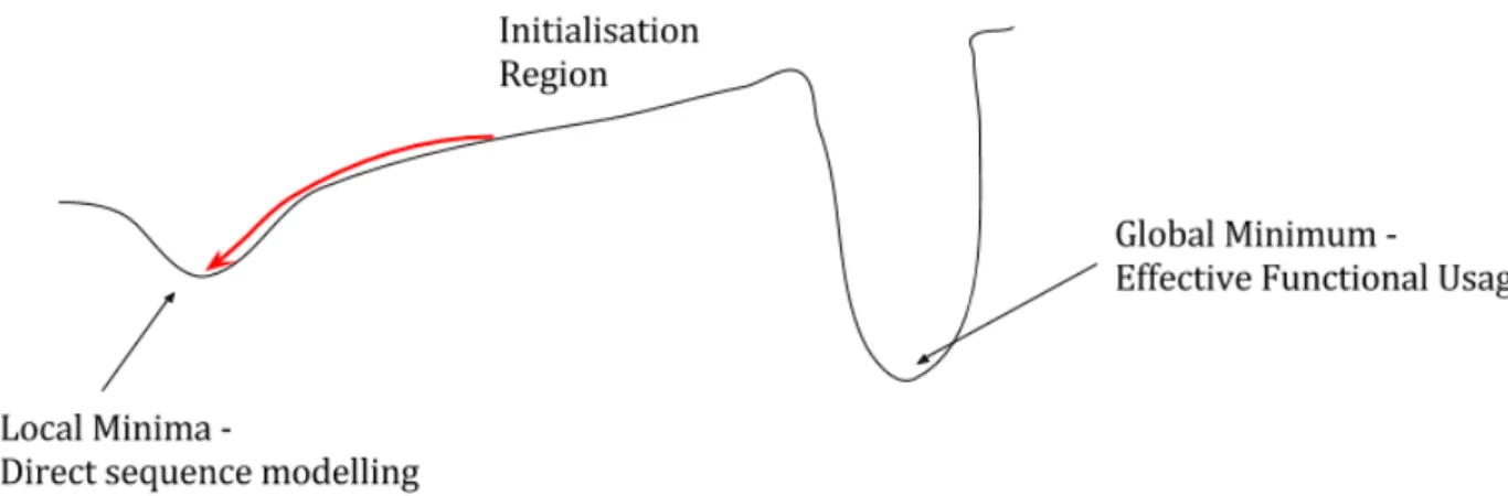
We therefore postulate that the weight space consists of two minima:

1. The most dominant corresponds to the region of weight-space in which the LSTMmodels the action sequence directly. This is a strong trajectory attractor where loss decreases rapidly, but fails to fully master the task as no function calls are made.

2. Theglobal minimais more elusive, occupying a region of weight-space in which configu-rations of LSTM parameters havelearnt to call the functions effectivelyand encapsulate behaviour. Since there are potentially more than one effective hierarchy, there could be multiple similar minima.

The space residing between these minima has a high loss, where the NPL simultaneously is learning when to call functions and what their form should be. We theorise that the random

(30)

12 A Marginal Loss Function

initialisation of LSTM parameters lies within the support basin of the strongly dominant local minima, preventing the functions from being learnt under weak supervision alone. Fully supervised pre-training, primes the NPL to learn from weak supervision by moving the LSTM to a point that lies within the support-basin of the global minima (See Figure 3.1 for a one-dimensional analogy).

Fig. 3.1 The weight-space problem, characterised by strongly attractive local minima that prevents the randomly initialised trajectories reaching the global minima.

3.1.2

Visualising Probability Propagation

To confirm or invalidate our belief we create animations of probability flow in the lattice by generating a matrix plot of yt_i,l yielding a frame for each time t. The recursive variable yt_i,l

quantifies the likelihood at each time step that the sum of latent execution paths has performed

i elementary operations correctly and is currently at depthl within the lattice. To convert our animations to an image, we sum along the time index, leading to Figure 3.2, in the presence of strong supervision. The probability flow is monitored at different points in training, both for trials using strong supervision and without. As expected in the fully supervised case, the probability flows through the lattice from left to right, dropping down into the second level as functions are called. In the absence of this strong supervision however, it is found that probability does not propagate further than the first elementary operation at any point in training, with only a sequence ofPOPorPUSHoperations observed (Figure 3.3). This is unexpected - as our weight-space hypothesis would suggest that probability mass flows through the lattice horizontally, but simply fails to call functions.

Flaws of the existing loss function

The observed phenomena has its origins in the loss function. The objective maximises the marginal probability of paths through the lattice that correctly perform allIelementary operations before callingPOPfrom the top level of the lattice. However, in order for this loss to be finite, a non-negligible degree of probability mass,yt_i,lmust reach the terminal node and subsequently callPOP. Due to random weight initialisation, the first training batch is extremely volatile with probability

(31)

3.2 A New, Local Objective 13

mass lost from paths thatPOP too early, call the wrong functions or PUSH too deeply into the hierarchy. The result is that no measurable probability mass reaches the terminal node indexI

yielding an infinite loss and a meaningless negligible gradient. This issue is notably absent in the presence of even a small amount of strong supervision as the pre-training biases the controller into a behaviour that is able to generate correct actions under subsequent weak supervision.

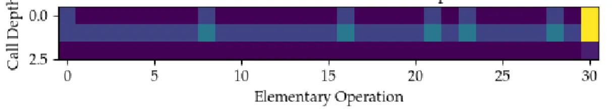
Fig. 3.2 A time-merged plot of yt_i,l probability flow through the lattice under fully supervised pre-training and the original loss function after 10,000 iterations. Colour intensity corresponds to higher values ofyt_i,l (summed acrosst). Training appears to have converged as there is only a single path, that successfully encapsulates all its actions within functions -shown by the majority of calls originating from the second level of the hierarchy. The pathPOPs to the top level before calling a new function withPUSH, returning to the second level. This is the behaviour we would hope to see inferred in the absence of strong supervision. This example is taken from theNanocraft

domain.

Fig. 3.3 Probability flow through the lattice under the original loss function in the absence of strong supervision. Note there is no horizontal flow ofy at all, with all probability mass lost through incorrect action calls orPOPPINGtoo soon.

3.2

A New, Local Objective

Evidently, the initialisation problem necessitates alocalform of loss to remain valid in the case of partially or even entirely incomplete action sequences. In deciding between candidate functions it is crucial that they:

1. Produce finite loss and usable gradients immediately, regardless as to the degree of probabil-ity mass reaching the terminal node.

2. EncouragePOPactions once allIof the elementary operations have been called.

Two alternatives to maximising the probability of an entire sequence - as done originally - would be to marginalise over elementary operationsior variable length sub-sequences beginning from

(32)

the initial indexi=0. These are investigated in turn, both producing workable gradients, with the former leading to more stable training.

3.2.1

Marginal Loss over Elementary Operations

The log likelihood can be written in marginal form:

log(P(λ0,λ1...λI)) = I

∑

i=0

log(P(λi)) (3.1)

To facilitate computation of this marginal loss, we redefine the recursive variableyt_i,las the proba-bility of generatingielementary operations either correctly or incorrectly (Eq. 3.2). Intuitively, this means that probability mass will flow through the lattice regardless as to whether or not the correct operation is called (as long as some operation ‘OP’ is called at all). See Figure 3.4

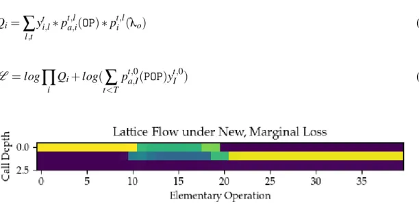
yt_i+1,l= p(OP)t_a,_,l_i₋₁yt_i,₋l₁+p(POP)t_a,_,l_i+1yt_i,l+1+p(PUSH)_at,_,l_i−1yt_i,l−1 (3.2) We define a variableQi, based on this new definition ofyt_i,las the probability of generating theith

elementary operation correctly, conditional on having generated the precedingi−1 elementary operations (either correctly or incorrectly). Philosophically, the lattice now learns to maximise the probability of each action independently, rather than the joint probability of the entire sequence. To encouragePOPoperations at the correct point in the lattice the original form of loss function is also included in the product for the final likelihood term. We refer to this reformulation as the marginal loss over elementary operations.

Qi=

∑

l,t yt_i_,_l∗pt_a,_,l_i(OP)∗pt_i,l(λo) (3.3) L =log

∏

i Q_i+log(

∑

t<T pt_a,_,0_I(POP)yt_I,0) (3.4)

Fig. 3.4 The time-merged lattice under the new, marginal loss function. Probability now propagates throughout the whole of the lattice, with latent paths making a function call at approximately the point where the nature of the task changes significantly (as will be seen in Section 3.3). This was not observed however during the greedy-decoding runs..

(33)

3.2 A New, Local Objective 15

3.2.2

Marginal Loss over Sub-Sequences of Elementary Operations

An alternate formulation of the loss is to marginalise over sub-sequences of correct elementary operations:

I

∑

j=0

log(P(λ0...λj)) (3.5)

Maximising the probability of longer chains of operations more closely reflects the original loss function. At test time a zero-one loss is used, meaning sequences of operations need be entirely correct to receive zero loss. In this formulationy is left as before, the probability of correctly

generating the precedingielementary operations (Equation 3.6).

yt_i+1,l=p(OP)t_a,_,l_i₋₁pt_o,_,l_i₋₁(λo)yt_i₋,l₁+p(POP)t_a,,li+1y t,l+1 i +p(PUSH) t,l−1 a,i y t,l−1 i (3.6)

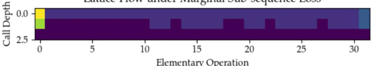
The variableQ_iremains identical to Equation 3.3 albeit with the original form ofy. We find that this form of loss leads to relatively unstable training curves, perhaps due to the over representation of initial elementary operations, present in each marginal term. Visualising lattice flow reveals that some functions of a single action are used, with the remainder called from the top level of the hierarchy (Figure 3.5).

Fig. 3.5 The time-merged lattice under the marginal sub-sequence loss. Probability flows through-out the lattice, with a portion of the latent paths calling functions and moving into the second level of the hierarchy. In greedy decoding, the controller LSTM calls only functions of a single action in length, corresponding to placing a block in theNanocraftdomain. As will be discussed in Section 3.3.

A Workable Gradient

Experiments from this point forwards are carried out using the marginal loss over elementary operations - defined with yt_i,l of the form in Equation 3.2. When trained under this new loss, probability is able to flow immediately through the lattice, with a workable gradient absent from initialisation problems of the original loss (Figure 3.6a).

(34)

(a)

(b)

Fig. 3.6 a) The evolution of clipped gradient during a training run in which fully supervised samples were present. Red corresponds to the average gradient of weakly supervised samplesunder the original loss function. Blue shows the mean gradient of the strongly supervised samples (trained with the loss function from NPI [9]). Note that gradient for the weak samples is zero at first before rising steadily as more probability mass reaches the terminal node due to the guidance from full supervision. b) The clipped gradient across three runs using entirely weak supervisionwith the new marginal loss function. Note that there is now a workable gradient immediately which slowly decreases as the model fits to the training data.

(35)

3.3 Nanocraft 17

3.3

Nanocraft

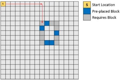
Nanocraft is an algorithmic toy task in which an agent must navigate through a 16x16 size grid-world in order to construct a rectangular ‘house’ of specified dimension, coordinates and material. The house has some pre-existing blocks but the agent must place the majority by executing a sequence of deterministic elementary operations: MOVE and PLACE (Figure 3.7). Each action requires arguments for specific directions or types of materials. An example execution trace, showing the abstract functions in bold is shown in the appendix (Figure A.1). Note that the presence of these abstract functions, such asBUILDWALL orMOVEMANYare not provided during training with weak supervision.

Fig. 3.7 TheNanocrafttask. The agent receives input from from three locations, the grid world embedding (from a convolutional encoder), a natural language embedding (specifying the type of house, size and location to build) and an embedding from the currently running program. Some blocks of the house are already placed in the grid. The agent must avoid placing blocks twice in the same location so needs to monitor the world state at all times.

3.3.1

Experiments

We repeat the experiments performed by Li et al. in [7], without any strong supervision. Despite the new marginal objective function - and decrease in training loss - it is found that held-out zero-one test loss does not decrease significantly or comparably with the results reported by Li et al.

Results

Marginal training loss is monitored alongside zero-one test loss, computed by performing a greedy decoding run on a batch of 500 held-out test samples and taking the mean of the binary scores. We find that training runs are volatile with differently seeded initialisations showing different convergence speeds and results (Figure 3.8). Curves are often grouped into two or three clusters where loss decreased slowly. Occasionally one of these curves will break from its group, with

(36)

loss decreasing rapidly until it either reaches the group below or successfully models the training data (registering near zero loss). Setting a limit on iteration number can therefore be difficult as one does not know if permitting training for slightly longer will lead to a sudden decrease in loss. We theorise that the presence of this phenomena is due to valleys in weight space or perhaps the segmented nature of the Nanocraft task, which consists of distinct sections of behaviour.

Training Curves

Fig. 3.8 The mean training curves, for 16, 32, 64, 128 and 512 weakly supervised samples. As indicated by the standard-deviation, training is highly volatile under gradient descent. There is a general trend that loss decreases most rapidly for those with the fewest numbers of samples as the network can rapidly adapt its parameters to fit the sequences. A minimum of two trials are performed in each case, with 512 and 128 repeated in greater number due to higher variation in results. Training loss here is the negative log-probability of calling the correct elementary operations independently and then callingPOPto terminate the algorithm.

(37)

3.3 Nanocraft 19

Fig. 3.9 The individual training runs performed with 512 weakly supervised samples. Note the fact that curves tend to follow one of three tracks possibly a result of different valleys in weight space.

Fig. 3.10 The training runs for the model with 16 Samples. Note that only one sample appears to fully explain the training data.

(38)

Analysis

The failure to generalise from the training samples stems from the controller modelling the action sequence directly, rather than encapsulating actions within functions. Indeed, only a single function was occasionally learned, in which the controller would place a single block before callingPOP. The advantage of this function seemingly that the model now has an additional time-step to evaluate whether a block need be placed or indeed if there is a pre-placed block in that location.

The percentage progression through the Nanocraft task was also recorded for each of the held out test samples. As one would expect, this increased with the degree of training data - Figure 3.11. TheQivalues from Equation 3.3 were averaged over each epoch and visualised. Notice that the

marginal probability of generating correct elementary operations evolves in line with the learning curves, there are sudden ‘jumps’ in the proportion ofQivalues that have high probability (Figure

3.12).

Fig. 3.11 The average progression of models trained under each number of samples through the

Nanocraft program. There is a clear trend for the progression to increase with the number of samples, as one would expect. The anomalous result for 128 samples reflects the volatility of the training process, with none of the performed trials completely fitting to the training samples in the allowed iterations.

(39)

3.4 Improving Training Stability 21

Q_iEvolution

(a) (b)

Fig. 3.12 A matrix plot ofQ_ivalues averaged over successive groups of 1000 iterations. Q_iis the marginal probability of generating theith elementary operation correctly, conditional on having generated the precedingi−1 elementary operations either correctly or incorrectly (Equation 3.3).

3.4

Improving Training Stability

The training process is computationally intensive for a single run, compounded by high volatility with identical hyper-parameters leading to different final results. The same features were exhibited in experiments by [7] and [9]. We looked at different approaches to alleviate this.

Scheduling Training Samples

We note that the error (and normalised gradient) of some training samples decreases to near zero relatively quickly - while others remain high. Rather than sampling the training data uniformly, we experiment with drawing samples in proportion to the magnitude of their average gradient. Similar approaches taken by [9] were found to decrease the number of iterations required for convergence. Unfortunately in practice, we find this often leads to less stable training curves so was not pursued (Figure 3.13).

Gradient Noise

Neelakantan et al. found in [8] that addition of Gaussian Noise to the gradients helped program induction, possibly by perturbing trajectories in weight space away from attractive modes. This was investigated but not found to make observable difference in our experiments.

(40)

Fig. 3.13 Trials using the scheduling procedure are found to be less stable - especially towards the end of training.

(41)

Chapter 4

Encouraging Hierarchy Use

Experiments in the previous chapter might suggest that gradient descent alone is insufficient to infer complex functional behaviour from observable actions. We seek to better understand whether this is the case and if the NPL framework could be used to learn functions when there is a very strong necessity to do so. We draw a dichotomy here between two groups of tasks that we refer to asworld dependantandworld independent. In both cases we find that the NPL only resorts to learning functions when all other forms of direct sequence to sequence learning are strongly penalised. Indeed, even when the hierarchy is used, functions inferred are not of the optimal form -with the model attempting to encapsulate actions in a single function that should be captured by two or three.

4.1

Recording and Constraining Hierarchy Use

One straightforward way to ensure that functions of some form are used would be to penalise long chains of elementary operations called from the same level of the hierarchy. This would account for the controller calling a single function and then modelling the entire process with the LSTM. To avoid the difficulties involved with measuringexpected function length1we instead measure theexpected number ofPUSH operations at each time step which we denoteζt2. To calculateζt

we note that the difference between the elementary operation indexiand the current time-stept

at any point within the lattice is equal to the number ofPUSH/POPcalls made during that path through the lattice. The number ofPUSH’s called is thus half this number (Equation 4.1).

ζt =

∑

i,l t−i 2 y t,l i (4.1)

1_{See the appendix for a less elegant way to constrain lattice flow}

2_{Note that the expected number of}_PUSH_{operations is identical to the expected number of functions from which} expected sequence lengthcan be calculated.

(42)

24 Encouraging Hierarchy Use

Enforcing MinimumPUSHCalls -β0

The first penalty we implement encourages the total expected number ofPUSHcalls to be equal to the actual number required, namely the number of functions called in generation of the synthetic sequence - n. We denote this penalty β0. The penalty is computed by taking square of the residual between the desired and actual number ofPUSHcalls at any point in training (Eq. 4.2). Implementation ofβ0alone leads to the model simply calling a sequence ofPUSH/POPoperations initially before modelling the entire sequence within a single program at the top of the hierarchy (Figure 4.1).

β0= (n−

∑

t

ζt)2 (4.2)

Fig. 4.1 Whenβ0is used alone, the model avoids proper use of function calls by simply calling several zero-length functions before modelling the actions as a sequence.

Enforcing Minimum Local Variance -β1

To prevent repeated length-zero function calls, thelocal variance v_w ofζ is computed, taking the

form of a modified 1D convolutional window that calculates variance - rather than a weighted sum - within each windoww(Eq. 4.3). We similarly defineβ1as the square of the residual betweenvw

and the true local variance, ˆv_w. Ideally, the values ofζt would be zero for elementary operations

(where the expected number ofPOPorPUSHcalls is zero) and 1 intermittently where the controller enters or returns from a function call. Hence the true value oflocalvariance will be high.

v_w=

∑

k∈w (ζk−µw)2 n−1 (4.3) β1=

∑

w (vˆ_w−v_w)2 (4.4)

Under constraints fromβ0andβ1, thePUSH/POPcalls are made with more appropriate spacing and frequency. However, the controller still avoids using the functions by performingPUSHbefore

(43)

4.1 Recording and Constraining Hierarchy Use 25

Fig. 4.2 When constrained through β0and β1 the controller avoids having to learn the correct program embeddings by calling the correct number ofPUSHandPOPoperations but in such a way as to still model the sequence as usual.

Enforcing Minimum Depth -β2

A final penalty is applied to restrict the expected depth of paths through the lattice. The expected depth,δ is calculated in (Eq. 4.5) with the target being the actual depth expected if the correct

number of functions are used. The loss applied is then the square of the difference between the true and expected depths, denotedβ2.

δ =

∑

i,t

lyt_i,l (4.5)

β2= (δˆ−δ)2 (4.6)

The combination of these three losses forces the NPL to call functions of approximately the right length without specifying exactly when functions must be called and for what purpose. Without any one of these, the functions would not be used.

Fig. 4.3 Whenβ0,β1andβ2are used the desired result is exhibited with functions of approximately constant length being called.

(44)

4.2

Bitflip

Bitflipis the name of a new task designed to analyse functional inference. The aim is to create an environment in which the gap between loss while using the hierarchy and that without is as large as possible. We consider several variations onBitflipwith the central theme involving an array of binary digits that must be manipulated according to the actively running program. We distinguish between the two forms of task set, referred to as;world dependantin the case where actions depend on the presence of theworld state w_t and world independent, in which actions only depend on the currently executed program. Using gradient descent alone in both cases leads to the top level program calling only elementary operations without use of the other levels. To avoid this we implement the three aforementioned penaltiesβ0,β1andβ2to force the calling of functions but allow the model flexibility to decide which programs are called and when.

World Independent Sequences

In the world independent paradigm, a set of patterns is generated (one for each callable function) and a sequence formed by concatenating the patterns in a random order. The order of patterns is shown at first before being obscured, forcing the LSTM to remember the order so as to execute it correctly (Figure 4.4 describes this in detail). The most efficient way to solve this task would be encapsulating each pattern within a single function and then calling in the order shown. Attempting to remember the sequence as a whole would mean larger parametric complexity within the hidden layer of the LSTM.

Fig. 4.4 Theworld independentBitflip environment. To generate the synthetic data, a set of latent functions (sequences) are generated (far left). These functions are then concatenated together repeatedly in a random order and this order is shown to the NPL at the start of program execution. The simplest way to solve the task is assigning a program embedding to model each of the latent functions and then calling these programs in the order shown originally.

World Dependant Sequences

In the world dependant case there exists an environmentw_t that the controller must manipulate according to the currently running function. This takes the form of an array of bits and a positional marker (Figure 4.5). The programs called now encapsulate abehaviour(orpolicy) rather than a simple fixed pattern of actions. We posit that this additional complexity could force the model into requiring the use of functions, especially if its LSTM hidden state was sufficiently small to lack the necessary capacity to model the behaviour directly.

(45)

4.3 Bitflip Results 27

Fig. 4.5World Dependant Bitflip the action sequence depends both on latent functions and the current state of the world. Random functions are again generated however in this case they representdesired behaviourrather than fixed patterns of actions. The currently running function dictates how the agent interacts with the value observed in the world grid. For example the random function - marked ‘0’ - is generated in the bottom of this diagram and indicates that when running, the action 2 should be called when a 0 is seen and 3 when a 1 is seen. A positional marker would also be present in the world grid to indicate where the agent is in the array of bits.

4.3

Bitflip Results

4.3.1

Learnt Functions

We carry out a set of experiments in both world independentandworld dependantdomains. Due to a non-linear rise in computational complexity with sequence length it is unfortunately not possible to consider long sequences where the use of functions would have greatest advantage. As a compromise, we restrict the controller to only 5 hidden units to remove as much capacity for direct sequence modelling as possible. We find that despite this, learning functions does not come naturally to the NPL with the controller strongly favouring use of one function (Figure 4.6). Analysis of the patterns produced by different functions after training has converged shows high variation between the output from a single function call (Table 4.1), suggesting the model is attempting to use one function to fit both patterns.

(46)

Learnt Function 1 Counts

3 10

blank 228

2,3,2,2 10

2, 3, 2, 3, 2 38

2, 2, 3, 2, 3, 2 38

Learnt Function 2 Counts

3, 2, 3, 2, 3 38

2, 3, 2, 2, 3 48

3, 3, 3, 2, 3, 3 10

blank 10

2, 2, 3, 3, 2, 3 10

Table 4.1 The actions performed when Functions 1 and 2 were called, alongside their frequency during the greedily decoded held-out data. These are the final form of the functions, before training terminated (Epoch 66) corresponding to Iteration 66000 in Figure 4.6. The true generative functions were2233and2323.

Fig. 4.6 We monitor the average number of each Function called during the greedy decoded runs performed on held-out data at the end of each epoch (1000 iterations). The controller rapidly learns to use a single function, minimising the three lattice penalties before adjusting slightly to call the second function more frequently. Training terminates when the loss decreases to zero for a set of consecutive iterations.

(47)

Chapter 5

Related Work

In recent years there has been a surge of interest in Augmented Neural Computation - the notion of endowing a fuzzy pattern matching neural machine with an external form of persistent manipulable memory [3]. This interest has stemmed primarily from the realisation that standard Recurrent Neural Networks (RNNs), including LSTMs are incapable of modelling certain simple, deterministic sequences1and fail to generalise to more than one task, suffering fromcatastrophic forgetting[5] [8] .

Neural Turing Machine (NTM)

The Neural Turing Machine proposed in [2] first showed that augmenting an LSTM with a manipulable read-write external memory lead to significant improvements in generalisation ability and enabled the machine to generalise to larger sequences than shown in training. The authors provided an LSTM controller with memory in the form of a matrix and attention-based, read/write heads. The focus and position of the heads could be tuned, and read/write operations were soft, making the system end-to-end differentiable and allowing the LSTM to attend to different parts of the memory. Results showed the NTM could infer basic algorithms from a limited number of input-output training examples.

Stack-Augmented RNN

The Stack-Augmented RNN model in [5] followed a different approach, endowing an LSTM controller with memory stacks to which it could optionally push its hidden state to or read from. It was demonstrated that these stacks enabled the model to perform deterministic sequence modelling tasks with very long dependencies. These tasks were not possible for a standard LSTM as the memory capacity of the hidden units was too small. The soft stack updates performed are similar to those performed at the lattice nodes of the NPL, as described in Chapter 2

(48)

30 Related Work

Neural Programmer Interpreter NPI

TheNeural Programmer Interpreter[9], is the direct predecessor to theNeural Program Lattice

on which this work is based. The NPI introduced the concept of a hierarchy of programs, that could be called by the LSTM controller. When called, the program’s embedding is fed as input to the LSTM in the proceeding time step. In this work, learning could only take place from fully supervised sequences of operations. That is, training data containing the full execution trace of both fundamental operations and abstract programs. The use of a program hierarchy allowed a single LSTM core to learn several distinct algorithmic tasks such as sorting, long addition and canonicalizing 3D models. Encapsulation of repeated behaviour allowed the NPI to achieve perfect generalisation after only 8 samples whereas a sequence-to-sequence model required 256. As discussed in Chapter 2, the Neural Program Lattice built on this work by enabling learning through mostly weak supervision.

Neural Programmer

Neelakantan et al. augment a neural network with a small set of basic arithmetic and logic operators, trainable with gradient descent. These operations can be called sequentially to compose higher order programs. The training data is unsupervised, avoiding expensive labelling and tasks considered include synthetic table comprehension questions consisting of question answer pairs. The authors note that training under purely weak supervision is challenging but found addition of Gaussian noise to the gradient to improve generalisation [8].

(49)

Chapter 6

Discussion

6.1

Conclusion

We set out to show that the Neural Program Lattice is capable of inferring a generative program hierarchy in the absence of hand-crafted supervision. Modification of the loss function enables learning, albeit without evidence of functional inference. Forcing the use of hierarchy through penalty terms on new, synthetic data shows that the NPL will use as few functions as possible to perform a given task, settling with one when two or three would be preferable. It thus would appear that our original weight-space hypothesis in Section 3.1.1 remains apt, with functional inference possible by the NPL but much less preferable to the strongly attractive region corresponding to sequence to sequence modelling by the LSTM controller in the top level of the hierarchy. Two statements seem fair to conclude with regards to the NPL and its predecessor the NPI:

1. The NPIlearnsandexecutesfunctions to great effect - enabling low sample complexity and strong generalisation.

2. The NPL is advantageous in thatgiven a pre-defined hierarchy, the provision of weakly supervised data enables significant performance increases from the NPI alone.

What is less clear, is whether the NPL can infer the hierarchy from elementary operations alone. Indeed, experiments in theBitflipdomain suggest this does not come naturally for the NPL in its current form, without pathological and seemingly over-engineered use of penalties. Cases in which the NPL would have a strong need to use functions, such as with very long sequence lengths are out of scope experimentally due to non-linear increases in computational complexity with the maximum length of sequence.

The core problem with inference in the NPL stems from the use of functions as a voluntary aid to the controller, rather than integral to the modelling process itself. In analogy with CNNs and RNNs where the weight-sharing component is fundamental to learning, the NPL/NPI is an LSTM with the added capacity for functionalexecution. The result is that program induction is not prioritised, with the LSTM controller preferring to stay in the top level of the hierarchy and focus on modelling the sequence directly.

(50)

32 Discussion

6.2

Future Work

Logical encapsulation and functional inference are arguably the next frontier of Deep Learning and form a natural next step to the existing hierarchies present in computer vision and time-series modelling. While it is difficult to suggest concrete re-formulations of the NPL to enable program induction, we offer two guiding principles for future work:

1. Learnt programs must be intrinsic to the modelling process, just as in a CNN the network is forced to compose lower level filters to form higher level features, so this should be the case with functional inference.

2. The inference procedure should have some form of localised learning ability, in the same way that an RNN can sequentially model a long text document, rather than having to observe the entire sequence as a whole.

Without changing the NPL, it would be interesting to see if a HMM or Hierarchical HMM [12] could be used to segment sequences of elementary operationsλ into clusters of similar behaviour

for use as approximate strong supervision. This could potentially bias the NPL towards learning more specific functions with further weak supervision.

(51)

References

[1] Badre, D. and Frank, M. J. (2012). Mechanisms of hierarchical reinforcement learning in cortico–striatal circuits 2: Evidence from fmri. Cerebral Cortex, 22(3):527–536.

[2] Graves, A., Wayne, G., and Danihelka, I. (2014). Neural tu