1 General Principles of Colloid Stability and the Role of Surface Forces

Tharwat Tadros

Abstract

In this overview, the general principles of colloid stability are described with some emphasis on the role of surface forces. Electrostatic stabilization is the re-sult of the presence of electrical double layers which, on approach of particles, interact, leading to repulsion that is determined by the magnitude of the surface or zeta potential and electrolyte concentration and valency. Combining this elec-trostatic repulsion with van der Waals attraction forms the basis of theory of col-loid stability due to Deyaguin-Landau-Verwey-Overbeek (DLVO theory). This the-ory can explain the conditions of stability/instability of colloidal particles and it can predict the Schulze-Hardy rule. Direct confirmation of the DLVO theory came from surface force measurements using cross mica cylinders. Particles containing adsorbed or grafted nonionic surfactant or polymer layers produce another mechanism of stabilization, referred to as steric stabilization. This arises from the unfavorable mixing of the stabilizing layers when these are in good solvent conditions and the loss of entropy of the chains on significant overlap. The criteria of effective steric stabilization have been summarized. The flocculation of sterically stabilized dispersions can be weak and reversible or strong and irreversible depending on the conditions. Weak flocculation can oc-cur when the adsorbed layer thickness is small (< 5 nm), whereas strong (incipi-ent) flocculation occurs when the solvency of the medium for the stabilizing chains become worse than that of a theta-solvent. The effect of addition of “free” non-adsorbing polymer is described in terms of the presence of a polymer-free zone (depletion zone) between the particles. This results in weak flocculation and equations are presented to describe the free energy of depletion attraction.

Colloids and Interface Science Series, Vol. 1

Colloid Stability: The Role of Surface Forces, Part I. Edited by Tharwat F. Tadros Copyright © 2007 WILEY-VCH Verlag GmbH & Co. KGaA, Weinheim ISBN: 978-3-527-31462-1

1

General Principles of Colloid Stability

and the Role of Surface Forces

1.1

Introduction

The stability of colloidal systems is an important subject from both academic and industrial points of views. These systems include various types such as sol-id–liquid dispersions (suspensions), liqusol-id–liquid dispersions (emulsions) and gas–liquid dispersions (foams). The colloid stability of such systems is governed by the balance of various interaction forces such as van der Waals attraction, double-layer repulsion and steric interaction [1]. These interaction forces have been described at a fundamental level such as in the well know theory due to Deryaguin and Landau [2] and Verwey and Overbeek [3] (DLVO theory). In this theory, the van der Waals attraction is combined with the double-layer repulsion and an energy–distance curve can be established to describe the conditions of stability/instability. Several tests of the theory have been carried out using mod-el colloid systems such as polystyrene latex. The results obtained showed the ex-act prediction of the theory, which is now accepted as the cornerstone of colloid science. Later, the origin of stability resulting from the presence of adsorbed or grafted polymer layers was established [4]. This type of stability is usually re-ferred to as steric stabilization and, when combined with the van der Waals at-traction, energy–distance curves, could be established to describe the state of the dispersion.

This overview summarizes the principles of colloid stability with particular reference to the role of surface forces. For more details on the subject, the read-er is refread-erred to two recent texts by Lyklema [5, 6].

1.2

Electrostatic Stabilization (DLVO Theory)

As mentioned above, the DLVO theory [2, 3] combines the van der Waals attrac-tion with the double-layer repulsion. A brief summary of these interacattrac-tions is given below and this is followed by establishing the conditions of stability/insta-bility describing the influence of the various parameters involved.

1.2.1

Van der Waals Attraction

There are generally two ways of describing the van der Waals attraction between colloids and macrobodies: the microscopic [7] and the macroscopic approach [8]. The microscopic approach is based on the assumption of additivity of London pair interaction energy. This predicts the van der Waals attraction with an accu-racy of *80%–90%. The macroscopic approach, which gives a more accurate evaluation of the van der Waals attraction, is based on the correlation between electric fluctuations of two macroscopic phases. However, this approach requires quantification of the dielectric dispersion data, which are available for only a

limited number of systems. For this reason, most results on the van der Waals attraction are based on the microscopic approach that is briefly described below. For a one-component system, individual atoms or molecules attract each other at short distances due to van der Waals forces. The latter may be considered to con-sist of three contributions: dipole–dipole (Keesom), dipole–induced dipole (Debye) and London dispersion interactions. For not too large separation distances be-tween atoms or molecules, the attractive energy Gais short range in nature and it is inversely proportional to the sixth power of the interatomic distance r:

Gaˆ b11

r6 …1†

whereb11is a constant referring to identical atoms or molecules.

Since colloidal particles are assemblies of atoms or molecules, the individual contributions have to be compounded. In this case, only the London interac-tions have to be considered, since large assemblies have no net dipole moment or polarization (both the Keesom and Debye forces which are vectors tend to cancel in such assemblies). The London (dispersion) interaction arises from charge fluctuations within an atom or molecule associated with the motion of its electrons. The London dispersion energy of interaction between atoms or molecules is short range as given by Eq. (1), wherebyb11 is now the London dispersion constant (that is related to the polarizability of atoms or molecules involved). For an assembly of atoms or molecules, as is the case with colloidal particles, the van der Waals energy of attraction between two equal particles each of radius R, at a distance h in vacuum, is given by the expression

GAˆ A11 6 2 s2 ₄‡ 2 s2‡ln s2 ₄ s2 …2† where s = (2R+h)/R and A11is the Hamaker constant, which is given by

A11ˆp2q2b11 …3†

where q is the number of atoms or molecules per unit volume.

For very short distances of separation (hR), Eq. (2) can be approximated by GAˆ RA11

12h …4†

It is clear from comparison of Eqs. (1) and (4) that the magnitude of the attractive energy between macroscopic bodies (particles) is orders of magnitude larger than that between atoms or molecules. It is also long range in nature, increasing sharp-ly at short distances of separation. GAis also proportional to R and A11.

The above expressions are for particles in vacuum and in the presence of a medium (solvent), the Hamaker constant A12of particles of material 1 dispersed in a medium of Hamaker constant A22is given by

A12ˆA11‡A22 2A12ˆ A 1 2 11 A 1 2 22 2 …5† Since with most disperse systems A11> A22 then a dispersion medium A12 is positive and two particles of the same material always attract each other.

The London dispersion forces exhibit the phenomenon of retardation implying that for large r the attraction decreases more rapidly with distance than at small r. This means that Ga (Eq. (1)) becomes proportional to r–7. For intermediate dis-tances there is a gradual transition from r–6to r–7[9]. This retardation is also re-flected in the attraction between particles, whereby h–1should be h–2 in Eq. (4). The retardation effect is automatically included in the macroscopic approach.

1.2.2

Double-layer Repulsion

Several processes can be visualized to account for charging suspended particles such as dissociation of surface groups (e.g. OH, COOH, SO4Na) and adsorption of certain ionic species (such as surfactants). In all cases, charge separation takes place with some of the specifically adsorbed ions at the surface forming a surface charge which is compensated with unequal distribution of counter and co-ions. This forms the basis of the diffuse double layer due to Gouy and Chap-man [10], which was later modified by Stern [11], who introduced the concept of the specifically adsorbed counter ions in the fixed first layer (the Stern plane). The potential at the surfacew0 decreases linearly to a value wd(located at the center of the specifically adsorbed counter ions) and then exponentially with de-crease in distance x, reaching zero in bulk solution. The Stern potential is sometimes equated with the measurable electrokinetic or zeta potential,f.

The extension of the double layer, referred to as double-layer thickness, de-pends on the electrolyte concentration and valency of the ions, as given by the reciprocal of the Debye-Hückel parameter:

1 jˆ ere0kT 2n0Z2e2 1 2 …6† whereer is the relative permittivity, e0 is the permittivity of free space, k is the Boltzmann constant, T is the absolute temperature, n0is the number of ions of each type present in the bulk phase, Z is the valency of the ions and e is the electronic charge.

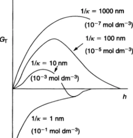
The parameter 1/j increases with decrease in electrolyte concentration and decrease in the valency of the ions. For example, for 1:1 electrolyte (e.g. KCl), the double-layer thickness is 100 nm in 10–5_{, 10 nm in 10}–3 _{and 1 nm in} 10–1_{mol dm}–3_{. As we shall see later, this reflects the double-layer repulsion, which} increases with decrease in electrolyte concentration.

When two particles each with an extended double layer with thickness 1/j approach to a distance of separation such that double-layer overlap begins to occur

(i.e. h < 2/j), repulsion occurs as a result of the following effect. Before overlap, i.e. h > 2/j, the two double layers can develop completely without any restriction and in this case the surface or Stern potential decays to zero at the mid-distance be-tween the particles. However, when h < 2/j, the double layers can no longer devel-op unrestrictedly, since the limited space does not allow complete potential decay. In this case the potential at the mid-distance between the particleswh/2is no long-er zlong-ero and repulsion occurs. The electrostatic enlong-ergy of repulsion, Gel, is given by the following expression which is valid forjR < 3:

Gelˆ

4pere0R2_w2

dexp… jh†

2R‡h …7†

Equation (7) shows that Gel decays exponentially with increase of h and it ap-proaches zero at large h. The rate of decrease of Gelwith increase in h depends on 1/j: the higher the value of 1/j, the slower is the decay. In other words, at any given h, Gelincreases with increase in 1/j, i.e. with decrease in electrolyte concentration and valency of the ions.

1.2.3

Total Energy of Interaction (DLVO Theory)

The total energy of interaction between two particles GTis simply given by the sum of Geland GAat every h value:

GTˆGel‡GA …8†

A schematic representation of the variation of Gel, GAand GTwith h is shown in Fig. 1.1. As can be seen, Gelshows an exponential decay with increase in h, ap-proaching zero at large h. GA, which shows an inverse power law with h, does not decay to zero at large h. The GT–h curve shows two minima and one maxi-mum: a shallow minimum at large h that is referred to as the secondary minimum, Gsec, a deep minimum at short separation distance that is referred to as the pri-mary minimum, Gprimary, and an energy maximum at intermediate distances,

Gmax (sometimes referred to as the energy barrier). The value of Gmax depends on the surface (Stern or zeta) potential and electrolyte concentration and valency. The condition for colloid stability is to have an energy maximum (barrier) that is much larger than the thermal energy of the particles (which is of the order of kT). In general, one requires Gmax> 25kT. This is achieved by having a high zeta potential (> 40 mV) and low electrolyte concentration (< 10–2mol dm–3 1:1 elec-trolyte). By increasing the electrolyte concentration, Gmax gradually decreases and eventually it disappears at a critical electrolyte concentration. This is illus-trated schematically in Fig. 1.2, which shows the GT–h curves at various 1/j values for 1:1 electrolyte. At any given electrolyte concentration, Gmaxdecreases with increase in the valency of electrolyte. This explains the poor stability in the presence of multivalent ions.

The above energy–distance curve (Fig. 1.1) explains the kinetic stability of col-loidal dispersions. For the particles to undergo flocculation (coagulation) into the primary minimum, they need to overcome the energy barrier. The higher the value of this barrier, the lower is the probability of flocculation, i.e. the rate of flocculation will be slow (see below). Hence one can consider the process of flocculation as a rate phenomenon and when such a rate is low enough, the sys-tems can stay stable for months or years (depending on the magnitude of the energy barrier). This rate increases with reduction of the energy barrier and ulti-mately (in the absence of any barrier) it becomes very fast (see below).

An important feature of the energy–distance curve in Fig. 1.1 is the presence of a secondary minimum at long separation distances. This minimum may

be-Fig. 1.1 Energy–distance curve for electrostatically stabilized systems.

Fig. 1.2 Energy–distance curves at various 1:1 electrolyte concentrations.

come deep enough (depending on electrolyte concentration, particle size and shape and the Hamaker constant), reaching several kT units. Under these condi-tions, the system become weakly flocculated. The latter is reversible in nature and some deflocculation may occur, e.g. under shear conditions. This process of weak reversible flocculation may produce “gels”, which on application of shear break up, forming a “sol”. This process of sol«gel transformation produces thixotropy (reversible time dependence of viscosity), which can be applied in many industrial formulations, e.g. in paints.

1.2.4

Stability Ratio

One of the useful quantitative methods to assess the stability of any dispersion is to measure the stability ratio W, which is simply the ratio between the rate of fast flocculation k0(in the absence of an energy barrier) to that of slow floccula-tion k (in the presence of an energy barrier):

Wˆk0

k …9†

The rate of fast flocculation k0was calculated by Von Smoluchowski [12], who con-sidered the process to be diffusion controlled. No interaction occurs between two colliding particles occurs until they come into contact, whereby they adhere irre-versibly. The number of particles per unit volume n after time t is related to the initial number n0by a second-order type of equation (assuming binary collisions):

nˆ n0

1‡k0n0t …

10† where k0is given by

k0ˆ8pDR …11†

where D is the diffusion coefficient, given by the Stokes-Einstein equation: Dˆ kT

6pgR …12†

Combining Eqs. (11) and (12): k0ˆ

8kT

6g …13†

For particles dispersed in an aqueous phase at 258C, k0= 5.5´10–18m3s–1. In the presence of an energy barrier, Gmax, slow flocculation occurs with a rate depending on the height of this barrier. In this case, a flocculation rate k

may be defined that is related to the stability ratio W as given by Eq. (9). Fuchs [13] related W to Gmaxby the following expression:

Wˆ2R Z1 2R exp Gmax kT h 2dh …14†

An approximate form of Eq. (14) for charge-stabilized dispersions was given by Reerink and Overbeek [14]:

Wˆ1 2k0exp Gmax kT …15† Reerink and Overbeek [14] also derived the following theoretical relationship be-tween W, electrolyte concentration C, valency Z and surface potentialw0:

log Wˆconstant 2:06109 Rc 2 Z2 log C …16† cˆexp…Zew0=2kT† 1 exp…Zew0=2kT† ‡1 …17†

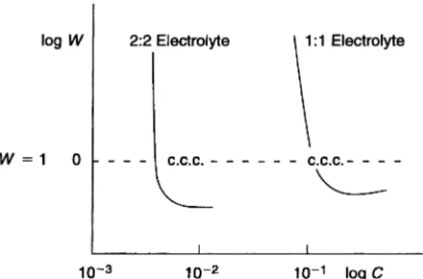
Equation (16) predicts that experimental plots of logW versus logC should be linear in the slow flocculation regime and logW = 0 (W = 1) in the fast floccula-tion regime. This is illustrated in Fig. 1.3 for 1 : 1 and 2 : 2 electrolytes. The plots show two linear portions intersecting at a critical electrolyte concentration at which W = 1, i.e. the critical flocculation concentration (CFC). Note that in Fig. 1.3, W is < 1 in the fast flocculation regime as a result of contribution of the van der Waals attraction.

Verwey and Overbeek [14] introduced the following criteria between stability and instability:

GTˆGel‡GAˆ0 …18† dGT

dh ˆ0 …19†

Using Eqs. (4) and (7), one can obtain an expression for the CFC: CFCˆ3:610 36 c

2

A2_Z2mol m

3 _20†

Equation (20) shows that the CFC increases withw0 or wdand decreases with increasing A (the Hamaker constant) or van der Waals attraction and it also de-creases with increase in Z. For very high values ofwd, capproaches unity and the CFC becomes inversely proportional to the sixth power of valency. However, very high values ofwdare not encountered in practice, in which case the CFC is proportional to Z–2_{. This dependence of CFC on Z is the basis of the} Schulze-Hardy rule.

As mentioned above, with electrostatically stabilized systems weak flocculation can occur, when a secondary minimum with sufficient depth (1–5kT) occurs in the energy–distance curve. In this case, the flocculation is reversible and in the kinetic analysis one must take into account the backward rate of flocculation (with a rate constant kb) as well as the forward rate of flocculation (with a rate constant kf). In this case the rate of decrease of particle number with time is given by

dn dt ˆ kfn

2_‡k

bn …21†

The rate of deflocculation kbdepends on the floc size and the exact ways in which the flocs are broken down (e.g. how many contacts are broken). This means that the second-hand term on the right hand-side of Eq. (21) should be replaced by a summation over all possible modes of breakdown, thus making the analysis of the kinetics complex. Another complication in the analysis of the kinetics of reversible flocculation is that this type of flocculation is a critical phenomenon rather than a chain (or sequential) process. Hence a critical particle number concentration, ncrit, has to be exceeded before flocculation occurs, i.e. flocculation becomes a thermo-dynamically favored process. The kinetics of weak, reversible flocculation have more in common, therefore, with nucleation kinetics, rather than with chemical (e.g. polymerization) kinetics. This is not to say that doublets, triplets, etc., will not form transiently below ncrit. These are thermodynamically unstable, but their effective concentrations may be calculated from a suitable kinetic analysis. This is beyond the scope of the present review.

The above flocculation process (strong or weak) is diffusion controlled and it is usually referred to as perikinetic flocculation. In other words, particle colli-sions arise solely from Brownian diffusion of particles and the diffusion coeffi-cient is given by the Stokes-Einstein relation D = kT/f, where f is the fractional

coefficient (as given by Eq. 12). If external energy is applied on the system, e.g. shear, ultrasound or centrifugal, or the system is not at thermal equilibrium (so that convection currents arise), then the rate of particle collisions is modified (usually increased) and the flocculation is referred to as orthokinetic. For exam-ple, in a shear field (with shear ratec), the rate of flocculation is given by

dn dtˆ

16 3 a

2_cR3 _22†

whereais the collision frequency factor, i.e. the fraction of collisions which re-sult in permanent aggregates. Although for irreversible flocculation one might expect orthokinetic flocculation conditions to lead to an increased rate of floccu-lation (in any given time interval), with a weakly (reversible) floccufloccu-lation the op-posite is the case, i.e. application of shear may lead to deflocculation.

1.2.5

Extension of the DLVO Theory

As discussed above, the basis premises of the DLVO theory are basically sound and considering van der Waals attraction and double-layer repulsion as the sole and additive contribution to the pair-wise interaction between particles in a dis-persion results in a number of predictions such as the dependence of stability on surface (or zeta potential), electrolyte concentration and valency (e.g. predic-tion of the Schulze-Hardy rule) as well as distincpredic-tion between “strong” (irrever-sible) flocculation and “weak” (rever(irrever-sible) flocculation. However, over the past five decades or so, a number of authors have attempted to extend the DLVO the-ory to take into account some of the unexplained results, e.g. the dependence of stability on the counter ion specificity (the so-called Hoffmeister series).

The main extension of the DLVO theory is the presence of repulsion at very short distances, which has been attributed to solvent structure-mediated forces (referred to as salvation forces). This will add an extra contribution to the pair-wise interaction, i.e.

GTˆGA‡Gel‡Gsolv;str …23†

For full consideration of the above extensions, one should refer to the recent text by Lyklema [15].

1.2.6

The Concept of Disjoining Pressure

The concept of disjoining pressure,P(h), was initially introduced by Deryaguin and Obukhov [16] to account for the stability of thin liquid films at interfaces. Basically, P(h) is the pressure that develops when two surfaces are brought to each other from infinity to a distance h. It is the change in the Gibbs free

en-ergy (in Joules) with separation distance h (in m). HenceP(h) is given as force per unit area (N m–2), which is the unit for pressure:

P…h† ˆ dG…h†

dh

p;T

…24†

P(h) can be split into three main contributions, PA (the van der Waals attrac-tion), Pel (the electrostatic repulsion) and Psolv,str (arising from salvation forces):

P…h† ˆPAPel‡Psolv;str …25†

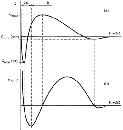
A schematic representation of the variation of G and P with h is shown in Fig. 1.4. The disjoining pressure diagram has three zero points at the secondary minimum, Gmax, and the primary minimum (at these points dG/dh = 0). How-ever, the zero mid-point (at the energy maximum) is not met in practice

be-Fig. 1.4 Gibbs free energy for the DLVO type of interaction between colloidal particles (top) and the corresponding disjoining pressure (bottom).

cause it is labile: a slight displacement to the right makesPpositive (repulsive), leading to further separation of particles.

The concept of disjoining pressure has been particularly useful in describing the stability of foam and emulsion films. Model foam films produced using ion-ic surfactants were used to describe the stability by measuring the disjoining pressure as a function of film thickness h [17]. The results obtained could be used to describe the mechanism of stabilization and hence to test the DLVO theory. The latter considers the interaction between parallel plates (the parallel layers of two surfactant films). In this case the electrostatic contribution to the disjoining pressure is given by

P…h†elˆ64RTC tanh2

Fw₀ 4RT

exp… jh† …26†

The van der Waals contribution to the disjoining pressure is given by P…h†vdWˆ

A

6ph3 …27†

Using Eqs. (26) and (27), one can calculate the total disjoining pressure P(h) and a direct comparison with the measured values can be obtained. This could prove the validity of the DLVO theory and any deviation could be accounted for by introducing other contributions, e.g. P(h)solv,st. Such comparison is beyond the scope of the present review.

1.2.7

Direct Measurement of Interaction Forces

There are generally two main procedures for measuring the interaction forces between macroscopic bodies, both of which have some limitations. The first technique is based on measurement of interaction forces between cross cylin-ders of cleaved mica (a molecularly smooth surface) that was described in detail by Israelachvili and Adams [18]. Full details of the technique are beyond the scope of this review. However, as an illustration, Fig. 1.5 shows the force–dis-tance curves for the interaction between two cross mica cylinders at various KNO3 concentrations. The semilogarithmic f(h) curves have a linear part, be-coming steeper with increasing salt concentration, corresponding to the long-distance exp(–jh) decay, predicted by the DLVO theory. For h < 2.5 nm, often a short-range repulsion is observed, which is due to the water structure-mediated solvation force.

The second technique for measuring interaction forces is based on atomic force microcopy (AFM), which will be described in detail in another chapter. In this technique, one can measure the force between a sphere and flat plate.

1.3

Steric Stabilization

This arises from the presence of adsorbed or grafted surfactant or polymer layers, mostly of the nonionic type. The most effective systems are those based on A–B, A–B–A block and BAn graft types (sometimes referred to as polymeric surfac-tants). Here B is the “anchor” chain that is usually insoluble in the dispersion me-dium and has strong affinity to the surface. A is the stabilizing chain that is sol-uble in the medium and strongly solvated by its molecules. To understand the role of these polymeric surfactants in the stabilization of dispersions, it is essential to consider the adsorption and conformation of the polymer at the interface. This is beyond the scope of the present review and the reader should refer to the text by Fleer et al. [19]. It is sufficient to state at this point that adsorption of polymers is irreversible and the isotherm is of the high-affinity type. The B chain produces small loops with multipoint attachment to the surface and this ensures irreversi-bility of adsorption. The stabilizing chains, on the other hand, extend from the sur-face, producing several “tails” with a hydrodynamic adsorbed layer thicknessdhof the order of 5–10 nm depending on the molecular weight of the A chains.

When two particles with radius R and having an adsorbed layer with hydrody-namic thicknessdhapproach each other to a surface–surface separation distance h that is smaller than 2dh, the polymer layers interact resulting in two main sit-uations [20, 21]: either the polymer chains may overlap or the polymer layer may undergo some compression. In both cases, there will be an increase in the local segment density of the polymer chains in the interaction zone. Provided that the dangling chains A are in a good solvent (see below), this local increase in segment density in the interaction zone will result in strong repulsions as a Fig. 1.5 Force–distance curves for two crossed mica cylinders at various KNO3concentrations.

result of two main effects: (1) increase in the osmotic pressure in the overlap re-gion as result of the unfavorable mixing of the polymer chains (when these are in good solvent conditions) [20, 21]; this is referred to as osmotic repulsion or mixing interaction and it is described by a free energy of interaction, Gmix; and (2) reduction of the configurational entropy of the chains in the interaction zone. This entropy reduction results from the decrease in the volume available for the chains whether these are either overlapped or compressed. This is re-ferred to as volume restriction interaction, entropic or elastic interaction and it is described by a free energy of interaction, Gel.

Combination of Gmixand Gelis usually referred to as the steric free energy of interaction Gs:

GsˆGmix‡Gel …28†

The sign of Gmix depends on the solvency of the medium for the chain. In a good solvent, i.e. the Flory-Huggins interaction parametervis < 0.5 (see below), then Gmixis positive and the unfavorable mixing interaction leads to repulsion. In contrast, ifv> 0.5, i.e. the chains are in poor solvent condition, then Gmixis negative and the interaction (which is favorable) is attractive. Gelis always posi-tive regardless of the solvency and hence is some cases one can produce stable dispersions in relatively poor solvent conditions.

Several sophisticated theories are available for description of steric interaction and these has been recently reviewed by Fleer et al. in a recent book by Lyklema [22]. However, in this section, only the simple classical treatment will be de-scribed, which is certainly an oversimplification and not exact.

1.3.1

Mixing Interaction, Gmix

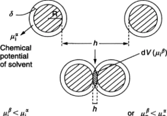
As mentioned above, this results from the unfavorable mixing of the polymer chains, when under good solvent conditions. This is represented schematically in Fig. 1.6, which shows the simple case of two spherical particles, each with radius R and each having an adsorbed layer with thicknessd. Before overlap, one can

de-Fig. 1.6 Schematic representation of polymer layer overlap.

fine in each polymer layer a chemical potential for the solventlia and a volume fraction for the polymer in the layer}2a. In the overlap region (volume element dV), the chemical potential of the solvent is reduced tolib; this results from the increase in polymer segment concentration in the overlap region (with a volume fraction}2b). This amounts to an increase in the osmotic pressure in the overlap region. As a result, solvent will diffuse from the bulk to the overlap region, thus separating the particles and, hence, a strong repulsive energy arises from this effect. The above repulsive energy can be calculated by considering the free energy of mixing two polymer solutions, as treated for example by Flory and Krigbaum [23]. This free energy is given by two terms: an entropy term that depends on the volume fraction of polymer and solvent and an energy term that is deter-mined by the Flory-Huggins interaction parameterv[24]:

d…Gmix† ˆkT…n1lny1‡n2lny2‡vn1y2† …29†

where n1and n2are the number of moles of solvent and polymer with volume fractions}1and}2, k is the Boltzmann constant and T is the absolute temperature. It should be mentioned that the Flory-Huggins interaction parameter v is a measure of the non-ideality of mixing a pure solvent with a polymer solution. This creates an osmotic pressurep that can be expressed in terms of the poly-mer concentration c2and the partial specific volume of the polymer (m2= V2/M2;

V2is the molar volume and M2is the molecular weight): p c2ˆRT 1 M2‡ m2 2 V1 1 2 v c2‡ …30† where V1is the molar volume of the solvent, R is the gas constant and T is the absolute temperature.

The second term in Eq. (30) is the second virial coefficient B2: p c2ˆ RT 1 M2‡ B2c2‡ …31† B2ˆ m 2 2 V1 1 2 v …32† Note that B2= 0 whenv= ½; the polymer behaves as ideal in mixing with the sol-vent. This is referred to as theh-condition. In this case the polymer chains in solu-tion have no attracsolu-tion or repulsion and they adopt their unperturbed dimension. Whenv< ½, B2is positive and mixing is non-ideal, leading to positive deviation (repulsion). This occurs when the polymer chains are in good solvent conditions. Whenv>½, B2is negative and mixing is non-ideal, leading to negative deviation (attraction). This occurs when the polymer chains are in poor solvent conditions. Using the Flory-Krigbaum theory and definition of the vparameter, one can derive the total change in free energy of mixing for the whole interaction zone by summing all the elements in dV:

Gmixˆ2kTV 2 2 V1 m2 1 2 v Rmix…h† …33†

wherem2is the number of chains per unit area and Rmix(h) is a geometric func-tion that depends on the form of the segment density distribufunc-tion of the chain normal to the surface,q(z).

Using the above analysis, one can derive an expression for the free energy of mixing of two polymer layers (assuming a uniform segment density distribution in each layer) surrounding two spherical particles as a function of separation distance h between the particles (21),

Gmix kT ˆ V2 2 V1 m2 1 2 v 3R 2d‡h 2 d h 2 2 …34† The sign of Gmix depends on the Flory-Huggins interaction parameter v: if v< ½, Gmixis positive and the interaction is repulsive; ifv> ½, Gmixis negative and the interaction is attractive. The conditionv= ½ and Gmix= 0 is termed the h-condition. The latter corresponds to the case where polymer mixing is ideal, i.e. mixing of the chains does not lead to either an increase or decrease of the free energy of the system. Theh-point represents the onset of change of repul-sion to attraction, i.e. the onset of flocculation (see below).

1.3.2

Elastic Interaction, Gel

As mentioned above, this arises from the loss of configurational entropy of the chain on the close approach of a second particle. This is represented in Fig. 1.7 for the simple case of a rod with one point attachment to the surface according to Mackor and van der Waals [25]. When the two surfaces are separated by an infinite distance (?), the number of configurations of the rod isX(?), which is proportional to the volume of the hemisphere swept by the rod. When a sec-ond particle approach to a distance h that such that it cuts the hemisphere (los-ing some volume), the volume available to the chain is restricted and the num-ber of configurations becomesX(h) which is less thanX(?).

For two flat plates, Gelis given by the expression

Gel kT ˆ2m2ln …h† …1† ˆ2m2Rel…h† …35†

where Rel(h) is a geometric function whose form depends on the segment den-sity distributionq(z).

Gelis always positive and could play a major role in steric stabilization. It be-comes very strong when the separation between the particles bebe-comes compar-able to the adsorbed layer thicknessd. It is particularly important for the case of multipoint attachment of the polymer chain.

1.3.3

Total Energy of Interaction

Combination of Gmixand Gelwith GA gives the total energy of interaction GT (assuming there is no contribution from any residual electrostatic interaction):

GTˆGmix‡Gel‡GA …36†

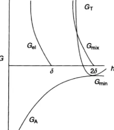
Figure 1.8 gives a schematic representation of the variation of Gmix, Gel, GAand

GTwith surface–surface separation h. Gmixincreases very sharply with decrease in h when h < 2d. Gelincreases sharply with decrease in h when h <d. GTversus

h shows only one minimum, Gmin, at h&2d. When h < 2d, GTshows a rapid in-crease with further dein-crease in h.

Unlike the GT–h curve predicted by the DLVO theory, which shows two mini-ma and one mini-maximum (see Fig. 1.4), the GT–h curve for sterically stabilized sys-Fig. 1.7 Scheme of configurational entropy loss on the approach of a second particle [25].

Fig. 1.8 Variation ofGmix,Gel,GAandGTwithh for a sterically stabilized system.

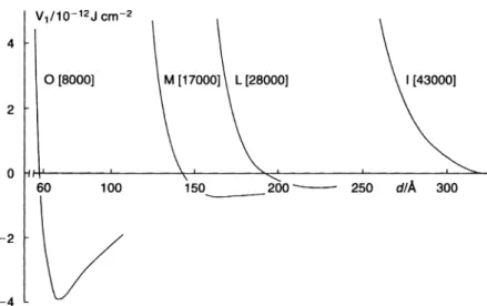
tems show only one shallow attractive minimum followed by a rapid increase in the total energy as the surfaces approach each other closely to distances compar-able to 2d. The depth of the minimum depends on the particle radius R, the Hamaker constant A and the adsorbed layer thickness d. For given R and A, Gmin increases with decrease ind, i.e. decreasing the molecular weight of the stabilizing chain. To illustrate this dependence, calculations were carried out for poly(vinyl alcohol) (PVA) polymer fractions with various molecular weights. The hydrodynamic thickness of these polymer fractions adsorbed on polystyrene la-tex particles was determined using dynamic light scattering [photon correlation spectroscopy (PCS)] and the results are given in Table 1.1.

Figure 1.9 shows the results of calculation for PVA of various molecular weight. As can be seen, Gmin increases with decrease in molecular weight. When the molecular weight of PVA is > 43 000, Gminis so small that it does not appear on the energy–distance curve. In this case, the dispersion will approach thermodynamic stability (particularly with low volume fraction dispersion). Fig. 1.9 Total interaction energy versus separation distance for particles

with adsorbed PVA layers of various molecular weights (thickness).

Table 1.1 Hydrodynamic thickness of PVA with various molecular weights.

MW d/nm 67000 25.5 43000 19.7 28000 14.0 17000 9.8 8000 3.3

However, when the molecular weight of the polymer reaches 8000 ordbecomes 3.3 nm, Gmin reaches sufficient depth for weak flocculation to occur. This was confirmed using freeze fracture scanning electron microscopy.

1.3.4

Criteria for Effective Steric Stabilization

1. The particles should be completely covered by the polymer, i.e. the amount of polymer should correspond to the plateau value. Any bare patches may cause flocculation either by van der Waals attraction between the bare patches or by bridging. The latter occurs when the polymer becomes simultaneously ad-sorbed on two or more particles.

2. The polymer should be strongly adsorbed (“anchored”) to the particle surface. This is particularly the case with A–B, A–B–A block and BAngraft copolymers where the B chain is chosen to be insoluble in the medium and has high af-finity to the surface. Examples of the B chain in aqueous media are polysty-rene and poly(methyl methacrylate).

3. The stabilizing chain A should be highly soluble in the medium and strongly solvated by its molecules, i.e. the Flory-Huggins interaction parameter v should remain < ½ under all conditions (e.g. in the presence of electrolyte and/or increase in temperature).

4. The adsorbed layer thicknessdshould be sufficiently large to maintain a shal-low minimum, Gmin. This is particularly the case when a colloidally stable dispersion without any weak flocculation is required. To ensure this colloid stability,dshould be > 5 nm.

1.3.5

Flocculation of Sterically Stabilized Dispersions 1.3.5.1 Weak Flocculation

This occurs when the thickness of the adsorbed layer thickness is small (usually < 5 nm), particularly when the particle size and Hamaker constant are large. In this case Gmin becomes sufficiently large (a few kT units) for flocculation to oc-cur. This flocculation is reversible and with concentrated dispersions the system may show thixotropy (at a given shear rate the viscosity decreases with time and when the shear is removed the viscosity increases to its initial value within a time-scale that depends on the extent of flocculation). This process, sometimes referred to as sol«gel transformation, is important in many industrial applica-tions, e.g. in paints and cosmetics.

The depth of the minimum, Gmin, required for flocculation depends on the volume fraction of the dispersion. This can be understood from a consideration of the free energy of flocculation,DGflocc, which consists of two terms, an en-thalpy term, DHflocc, which is negative and determined by the magnitude of

Gmin, and an entropy term, TDSflocc, which is also negative since any aggrega-tion results in a decrease in entropy. According to the second law of thermody-namics

DGflocc_ˆDHflocc _TDSflocc _37†

Hence the second term in Eq. (37), which has a negative sign, becomes positive and therefore entropy reduction must be compensated by a high enthalpy term for flocculation to occur, i.e. forDGfloccto become negative.

For a dilute dispersion with a low volume fraction}, the entropy loss on floc-culation is large, and to obtain an overall negative free energy,DHfloccneeds to be large, i.e. a large Gminis required. In contrast, for a concentrated dispersion with large }, the entropy loss on flocculation is relatively small and a lower Gmin is sufficient for flocculation to occur. This means that Gmin required for flocculation decreases with increase in the volume fraction}of the dispersion.

1.3.5.2 Strong (Incipient) Flocculation

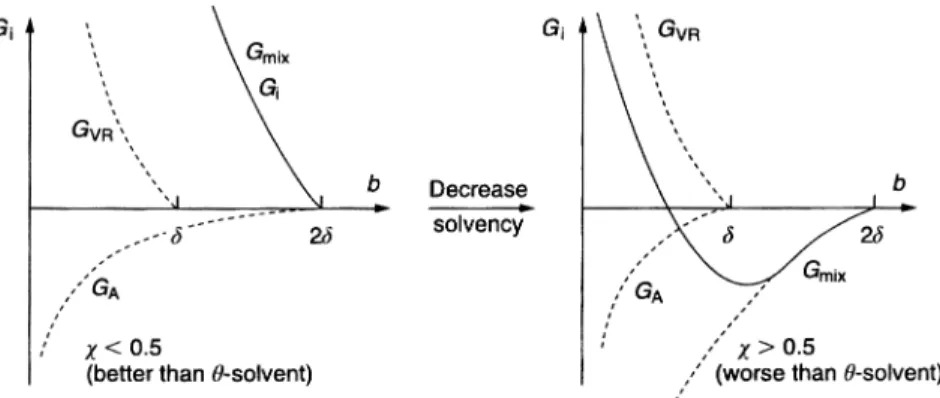
This occurs when the solvency of the medium for the chains becomes worse than ah-solvent, i.e.v> ½. This is illustrated in Fig. 1.10, which shows the situa-tion when vchanges from a value < ½ for a good solvent to > ½ for a poor sol-vent. When v< ½, both Gmixand Gel(or GVR) are positive and hence the total energy of interaction will show only a shallow minimum at a distance close to 2d. However, whenv> ½, Gmixbecomes negative (attractive), which, when com-bined with the van der Waals attraction, gives a deep minimum causing “cata-strophic” flocculation, usually referred to as incipient flocculation. In most cases, there is a correlation between the critical flocculation point and theh -con-dition of the medium. Good correlation is found in many cases between the critical flocculation temperature (CFT) and h-temperature of the stabilizing

Fig. 1.10 Influence of reduction in solvency of the medium for the chains on the energy–distance curve for sterically stabilized dispersions.

chain A in solution. Good correlation is also found between the critical volume fraction (CFV) of a non-solvent for the A chain and its h-point. However, in some cases such correlation may break down, particularly the case for polymers that adsorb with multi-point attachment. This situation has been described by Napper [20], who referred to it as “enhanced” steric stabilization.

Hence by measuring the vparameter for the stabilizing chain as a function of the system variables such as temperature and addition of electrolytes, one can establish the limits of stability/instability of sterically stabilized dispersions. Thevparameter can be measured using various techniques, e.g. viscosity, cloud points, osmotic pressure or light scattering.

1.4

Depletion Flocculation

This is produced on the addition of “free”, non-adsorbing polymer to a disper-sion [26]. The free polymer cannot approach the particle surface by a distanceD (that is approximately equal to twice the radius of gyration of the polymer, 2RG). This is due to the fact that when the polymer coils approach the surface, they lose entropy and this loss is not compensated by an adsorption energy. Hence the particles will be surrounded by a depletion zone (free of polymer) with thicknessD. When the two particles approach each other to a surface–sur-face separation distance < 2D, the depletion zones of the two particles will over-lap. At and above a critical volume fraction of the free polymer}p+, the polymer coils become “squeezed” out from between the particles and hence the osmotic pressure outside the particle surfaces becomes higher than in between them (with a polymer-free zone) and this results in weak flocculation. The first quan-titative analysis of this process was carried out by Asukara and Osawa [26], who derived the following expression for the depletion free energy of attraction:

Gdepˆ 3 2y2bx

2_{; 0<x<1 …38†}

where}2is the volume concentration of the free polymer:

y2ˆ 4 3pD 3_N 2 V …39†

N2is the total number of coils and V is the volume of solution.bis equal to R/D and x is given by

xˆD …h=2†

Fleer et al. [27] derived the following expression for Gdep: Gdepˆ l1 l 0 1 V1 2p 3 D 1 2h 2 3R‡2D‡1 2h …41† wherel10_{andl1are the chemical potentials of pure solvent and polymer} solu-tion with a volume fracsolu-tion}pand V1is the molar volume of the solvent.

References

1 Th. F. Tadros (ed.), Solid/Liquid

Disper-sions, Academic Press, London (1987).

2 B. Deryaguin and L. D. Landau, Acta

Physicochim. USSR, 14, 633 (1941).

3 E. W. Verwey and J. Th. G. Overbeek,

Theory of Stability of Lyophobic Colloids,

Elsevier, Amsterdam (1948).

4 D. H. Napper, Polymeric Stabilization of

Colloidal Dispersions, Academic Press,

London (1983).

5 J. Lyklema, Fundamentals of Interface and

Colloid Science, Vol. I, Academic Press,

London (1991).

6 J. Lyklema, Fundamentals of Interface and

Colloid Science, Vol. II, Academic Press,

London (1995).

7 H. C. Hamaker, Physica (Utrecht), 4, 1058 (1937).

8 E. M. Lifshits, Sov. Phys. JETP, 2, 73 (1956). 9 H. B. G. Casimir and D. Polder, Phys.

Rev., 73, 360 (1948).

10 G. Gouy, J. Phys., (4) 9, 457 (1910); Ann.

Phys., (9) 7, 129 (1917); D. L. Chapman, Philos. Mag., (6) 25, 475 (1913).

11 O. Stern, Z. Electrochem., 30, 508 (1924). 12 M. Von Smoluchowski, Phys. Z., 17, 557,

585 (1917).

13 N. Fuchs, Z. Phys., 89, 736 (1934). 14 H. Reerink and J. Th. G. Overbeek,

Discuss. Faraday Soc., 18, 74 (1954).

15 J. Lyklema, Fundamentals of Interface and

Colloid Science, Vol. III, Academic Press,

London (2000).

16 B. V. Deryaguin and E. Obukhov, Zh. Fiz.

Khim., 7, 297 (1936).

17 D. Exerowa and P. M. Kruglyakov, Foam

and Foam Films, Studies in Interface

Science, Vol. 5, Elsevier, Amsterdam (1998).

18 J. N. Israelachvili and G. E. Adams,

J. Chem. Soc., Faraday Trans. 1, 74, 975

(1978).

19 G. J. Fleer, M. A. Cohen Stuart, J. M. H. M. Scheutjens, T. Cosgrove and B. Vincent, Polymers at Interfaces, Chap-man and Hall, London (1993).

20 Th. F. Tadros and B. Vincent, in

Encyclo-pedia of Emulsion Technology, P. Becher

(ed.), Marcel Dekker, New York (1983). 21 Th. F. Tadros, in Principles of Science and

Technology in Cosmetics and Personal Care,

E. D. Goddard and J. V. Gruber (eds.), 73–113. Marcel Dekker, New York (1999). 22 J. Lyklema, Fundamentals of Interface and

Colloid Science, Vol. V, Elsevier,

Amster-dam (2005).

23 P. J. Flory and W. R. Krigbaum, J. Chem.

Phys., 18, 1086 (1950).

24 P. J. Flory, Principles of Polymer Chemistry, Cornell University Press, Ithaca, NY (1953).

25 E. L. Mackor and J. H. van der Waals,

J. Colloid Sci., 7, 535 (1951).

26 A. Asukara and F. Oosawa, J. Chem.

Phys., 22, 1235 (1954); J. Polym. Sci., 93,

183 (1958).

27 G. J. Fleer, J. M. H. M. Scheutjens and B. Vincent, Am. Chem. Soc. Symp. Ser.,