Robot Navigation in Cluttered Environments with Deep Reinforcement Learning

(1)

ROBOT NAVIGATION IN CLUTTERED ENVIRONMENTS WITH DEEP REINFORCEMENT LEARNING

A Thesis presented to

the Faculty of California Polytechnic State University, San Luis Obispo

In Partial Fulfillment

of the Requirements for the Degree Master of Science in Electrical Engineering

by

Ryan Weideman June 2019

(2)

(3)

COMMITTEE MEMBERSHIP

TITLE: Robot Navigation in Cluttered Environ-ments with Deep Reinforcement Learning

AUTHOR: Ryan Weideman

DATE SUBMITTED: June 2019

COMMITTEE CHAIR: John Seng, Ph.D.

Professor of Computer Science

COMMITTEE MEMBER: Helen Yu, Ph.D.

Professor of Electrical Engineering

COMMITTEE MEMBER: Vladimir Prodanov, Ph.D.

(4)

ABSTRACT

Robot Navigation in Cluttered Environments with Deep Reinforcement Learning Ryan Weideman

The application of robotics in cluttered and dynamic environments provides a wealth of challenges. This thesis proposes a deep reinforcement learning based sys-tem that determines collision free navigation robot velocities directly from a sequence of depth images and a desired direction of travel. The system is designed such that a real robot could be placed in an unmapped, cluttered environment and be able to navigate in a desired direction with no prior knowledge. Deep Q-learning, coupled with the innovations of double Q-learning and dueling Q-networks, is applied. Two modifications of this architecture are presented to incorporate direction heading in-formation that the reinforcement learning agent can utilize to learn how to navigate to target locations while avoiding obstacles. The performance of the these two ex-tensions of the D3QN architecture are evaluated in simulation in simple and complex environments with a variety of common obstacles. Results show that both modifica-tions enable the agent to successfully navigate to target locamodifica-tions, reaching 88% and 67% of goals in a cluttered environment, respectively.

(5)

ACKNOWLEDGMENTS

Thanks to:

• Dr. Seng for advising me on this project

• My family for supporting me always, and for providing delicious home-made orange juice

(6)

LIST OF TABLES

Table Page

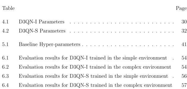
4.1 D3QN-I Parameters . . . 30 4.2 D3QN-S Parameters . . . 32 5.1 Baseline Hyper-parameters . . . 41 6.1 Evaluation results for D3QN-I trained in the simple environment . 54 6.2 Evaluation results for D3QN-I trained in the complex environment 54 6.3 Evaluation results for D3QN-S trained in the simple environment . 56 6.4 Evaluation results for D3QN-S trained in the complex environment 57

(9)

LIST OF FIGURES

Figure Page

1.1 High level overview of the reinforcement learning system developed 3

2.1 Agent-Environment interaction from [1] . . . 5

2.2 Perceptron model of a neuron . . . 10

3.1 Original Deep Q-Network proposed in [14] . . . 18

3.2 Dueling Q-network Architecture [16] . . . 20

4.1 System overview . . . 23

4.2 Example stack of four 160x128 depth images taken following random policy, wheret = 3 is the current depth image . . . 25

4.3 Robot Heading and Goal . . . 26

4.4 D3QN architecture for playing Atari games. . . 28

4.5 D3QN-I architecture . . . 30

4.6 D3QN-S architecture . . . 31

5.1 Turtlebot Model . . . 36

5.2 Example obstacles captured in depth images . . . 39

5.3 Simple Training Environment . . . 40

5.4 Complex Training Environment . . . 40

5.5 Simple evaluation environment, average path length 8.18 meters . . 43

5.6 Complex evaluation environment, average path length 8.4 meters . 43 6.1 Simple environment training results . . . 46

6.2 Longer training average reward results . . . 48

6.3 Percentage goals reached in simple training environment . . . 48

6.4 Complex environment training results . . . 49

6.5 D3QN-S trained for 1,600,000 steps in the complex environment . . 50

(10)

6.7 Example stack of four 80x64 depth images from complex environ-ment, t= 3 is the current depth image, the goal is 15.2◦ to the left, obtained following a random policy . . . 51 6.8 Q-value analysis for D3QN-I with 80x64 resolution images . . . 52 6.9 D3QN-I action distribution . . . 55 6.10 Four example paths from the simple evaluation environment. Green

circles represent starting locations. Red circles represent goal loca-tions. Red paths were taken by D3QN-I. Blue paths were taken by D3QN-S. . . 58 6.11 Four example paths from the complex evaluation environment. Green

circles represent starting locations. Red circles represent goal loca-tions. Red paths were taken by D3QN-I. Blue paths were taken by D3QN-S. . . 59

(11)

LIST OF ALGORITHMS

1 Q-Learning . . . 9 2 Deep Q-learning with Experience Replay Pseudo-Code . . . 33

(12)

Chapter 1 INTRODUCTION

Autonomous mobile robots are becoming increasingly prevalent in everyday life. Although robots have seen wide spread industrial application since the 1970’s, robots are starting to see applications in other less controlled and complex domains such as delivery, the home, medical, military, entertainment, and dangerous environments that humans cannot enter. Extension into these new domains presents a wealth of new challenges.

This thesis explores the challenge of autonomous mobile robot navigation in com-plex environments. The objective of autonomous mobile robot navigation is to achieve safe and efficient travel from one location to another, without colliding with obstacles. This could be for all types of robots, however this thesis is concerned with robots that move laterally throughout buildings and other cluttered spaces. Navigation in such complex environments traditionally requires a map of the environment, continuous localization of the robot within that environment using a multitude of sensors, and pathfinding algorithms that utilize knowledge of the map and the dynamics of the robot to generate paths that can be feasible traversed. The algorithms behind this multipronged approach require a large number of manually tuned parameters, and the behavior of the robot is often difficult to specify for complex scenarios.

Deep reinforcement learning is applied in this thesis to instead have a robot learn how to behave by repeatedly interacting with its environment, much like how humans learn through accumulated life experiences. Additionally, the system is designed to use information that a human has when determining how to navigate. The system uses a depth camera sensor to obtain information about the robot’s surroundings, and a simple angle representing the desired direction of travel, much like how a human

(13)

knows what direction they desired to move in. The pipeline from sensor input to robot controls is simplified into an end-to-end model that is represented by a deep neural network, rather than a collection of algorithms that require manual tuning.

1.1 Contributions

This thesis focuses on applying reinforcement learning and neural networks to the problem of determining navigation behaviors for mobile autonomous robots. The primary contributions are as follows:

1. Applies Q-learning to determine robot controls solely from a sequence of depth images and a desired direction input

2. Introduces two modifications of the D3QN architecture to fuse depth images and direction input

3. Evaluates performance of the proposed models in simple and complex navigation scenarios in simulation

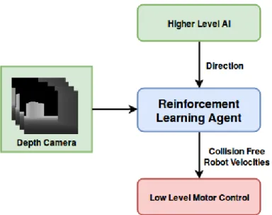
The system presented in this thesis is designed to simplify the task of generating feasible navigation controls for the robot to follow. A higher level form of control feeds into the system the desired direction, such as the direction toward a tracked target object with an RGB camera, along with a sequence of depth images to produce robot velocity commands that result in safe and efficient travel toward the desired position. Figure 1.1 illustrates an overview of this system.

(14)

Figure 1.1: High level overview of the reinforcement learning system de-veloped

The designed model is implemented for a robot called Turtlebot, which is a robot commonly used in robotics research that features a differential drive train and a 3D depth camera. The Robot Operating System (ROS) is leveraged as a platform for running the software developed to implement the model, coupled with open-source robotics simulator Gazebo for training the model with suitably accurate physics and depth camera sensor simulation.

This document is broken down into the following. Firstly in Chapter 2, the essen-tial foundational background theory behind reinforcement learning and neural net-works is outlined. Following in Chapter 3 is a discussion work related to autonomous navigation, including the traditional method of mapping, localizing, and path plan-ning, and the primary research in Q-learning that the system in this thesis is built off of. Chapter 4 outlines the design of the system, followed by Chapter 5 which elabo-rates how the system was implemented and what software tools were used. Chapter 6 shares the experimental results of the method and includes an analysis of its perfor-mance. Finally, Chapter 7 outlines how the system could be improved and extended, followed by concluding thoughts in Chapter 8.

(15)

Chapter 2 BACKGROUND

This thesis focuses primarily on the application of neural networks and reinforce-ment learning to the problem of autonomous robot navigation and obstacle avoid-ance. This chapter will first begin with an overview of reinforcement learning and the specific class of algorithm applied in this thesis, followed by an overview of neural networks, and finally concludes with an overview of depth sensing.

2.1 Reinforcement Learning

Reinforcement learning is a unique machine learning paradigm. It differs from supervised learning where the input and output of the model is already known, and the model is trained to generalize from that labeled data, and different from unsupervised learning, where the desired output of the model is unknown but the model finds patterns in the data. Reinforcement learning algorithms fit into neither of these classes; they do not have direct supervision or a complete model of the environment but instead gain experience from repeatedly interacting with the environment, with a reward signal as feedback for the model’s performance. The objective of the agent is to maximize the reward signal over time.

The framework used to describe reinforcement learning algorithms is very abstract. The model that learns the desired behavior is called an agent, and that agent learns by interacting with its environment. In general, anything that cannot be changed by the agent is considered part of the environment [1]. At each time-step t, the agent has an understanding of the environment in the form of stateSt ∈ S, whereS is the set of all possible states. The state of a reinforcement learning problem can be nearly

(16)

anything that would help the agent decide what actions to take: images, sensor data, abstract features, words, etc. The agent uses state St to decide what action At ∈ A to take, where A is set of all actions that can be taken in state St. Actions are also very general; they can be low level motor voltages or high level commands, such as go to a specific location. Upon taking the action, the agent receives feedback in the form of reward Rt+1, which is single numerical value. The reward is positive if action At was determined to be a good action or negative if it was a bad action. The agent also receives the next state St+1 from the environment, and the process repeats. Figure

2.1 illustrates this interaction between agent and environment.

Figure 2.1: Agent-Environment interaction from [1]

Most reinforcement learning problems are assumed to meet the Markov property, which states that future states depend only the current state and not the preceding states. This assumes that the knowledge contained in the current state is a good basis for estimating future rewards and selecting the best actions [1]. Making the Markov assumption also allows reinforcement learning problems to mathematically formalized as Markov Decision Processes (MDP), which are defined by their states, actions, and the probabilities of the transitions between states. When reinforcement learning problems are described by MDPs, it is possible to predict all future states and rewards from any given state. Thus, its best to select the state in a reinforcement learning problem to satisfy the Markov property as much as possible. Solving an MDP

(17)

refers to finding the best policy π, where a policy is what determines what action to take in any given state.

The value of any state is a measure of how ”good” it is to be in that state. It defined as the expected sum of discounted future rewards progressing from that state under a policy π, see eq. (2.1). Gt in eq. (2.1) describes the sum of discounted re-wards, whereγ is the discount factor. A discount factor close to one would mean that rewards far off in the future are weighted similarly to short term rewards, whereas a smaller discount factor makes the agent more shortsighted, caring only about rewards in the near future.

Gt = ∞ X k=0 γkRt+k+1 (2.1) 0≤γ ≤1 (2.2) vπ(s) =Eπ[Gt |St =s] (2.3) Similar to the state-value function, the action-value function for policy π can be described with eq. (2.4). This is the sum of discounted rewards if the action a is taken from state s and policy π is followed. The action-value of state s and action a is commonly referred to as the Q-value of that state action pair.

qπ(s, a) = Eπ[Gt|St=s, At=a] (2.4)

2.1.1 Optimal Policy

The optimal policy of a reinforcement learning problem describes the best action to take in any given state. If the optimal policy is known, then that problem is solved, since taking the highest valued action in each state will ultimately maximize reward. For smaller Markov decision processes where the dynamics of the environ-ment are completely known, then the optimal policy can be found through dynamic programming techniques. However, for scenarios where the dynamics of the

(18)

envi-ronment are not completely known and the state and action spaces are very large, which is most reinforcement learning problems, finding the exact optimal policy is not directly possible with dynamic programming techniques. Thus, the objective of most reinforcement learning algorithms is to best approximate the optimal policy. The optimal policy π∗ has the optimal state-value function

v∗(s) = max

π vπ(s) = maxπ Eπ[Gt |St=s] (2.5) for all states s. The optimal policy is the policy that finds itself in states that maximize the expected value of the discounted sum of future rewards. Similarly, the optimal policy has the optimal action-value function

q∗(s, a) = max

π qπ(s, a) = maxπ Eπ[Gt |St =s, At=a] (2.6) The optimal policy will maximize the expected the expected value of the dis-counted sum of future rewards if action a is taken in state s. If the optimal action-value function q∗(s, a) is known, obtaining the optimal policy is trivial. In each state the agent finds itself in, it simply takes the action with the highest q-value. Tak-ing this action at each state would successfully maximize the reward received by the agent.

2.1.2 Q-Learning

The objective of Q-learning is to iteratively approximate the optimal action-value function q∗, eq. (2.6). Q-Learning is a type of temporal difference learning, which uses the current action-value function estimate to bootstrap and estimate an updated action-value function. It is a type of model-free reinforcement learning, in which there is no model of the environment, thus it learns a solution to the Markov decision process describing the problem without knowing the transition probabilities between states. This makes Q-learning particularly powerful for solving reinforcement learning problems, since the environment is often very difficult if not impossible to model.

(19)

Q-learning works by iteratively visiting states of the MDP and re-estimating the action-value function, denotedQ(s, a), using the previous action-value function values for that state. Equation (2.7) outlines the process of updating the Q function for a given state and action after taking that action and observing the results.

Q(st, at)←Q(st, at) +α[rt+1+γmax

a Q(st+1, a))−Q(st, at)] (2.7) Q-learning is considered an off-policy algorithm because the update to the Q function, [rt+1 +γmaxaQ(st+1, a))− Q(st, at)], uses the q-value of the maximum valued action of the next state, as opposed to the action that would actually be taken following the current policy π. This has the effect of directly approximating the optimal policy, as desired. The value α is the scalar weighting of how much the update should effect the Q-function.

The action selected in each state is the action that has the highest q-value, argmax_aQ(st, a). However, there is an issue with this during the learning of the Q-function. If the maximum q-valued action is taken at every time step, actions that have not been previously taken or that were previously estimated low-value, may actually have higher value than the current max valued action. The result is that the optimal Q-function will not be learned, since it failed to take the actual highest valued action. The solution is to have the agent explore its Q-function by occasion-ally taking actions that are not max-valued, so that the Q-function is updated for all actions. This is typically implemented as−greedy, which is where at each time step, there is a probability of a random action a∈ A being taken. This problem is com-monly referred to in reinforcement learning literature as the problem of exploration vs. exploitation.

(20)

Algorithm 1 Q-Learning

InitializeQ(s, a),∀s∈ S,∀a∈ A(s), arbitrarily, andQ(terminal,·) = 0 for each episodedo

Initialize s

for each step of episode do

Choose a froms using policy derived from Q (eg. -greedy) Take action a, observe r,s0

Q(st, at)←Q(st, at) +α[rt+1+γmaxaQ(st+1, a))−Q(st, at)] s←s0

Until S is terminal end for

end for

For small MDPs, the Q-function can be represented as a simple table, where the Q-value for each state and action is maintained in the table for easy lookup. For complex problems with large state and action spaces, however, tabular methods do not work as the table would become too large and there would be too many unique state-action pairs to visit to successfully populate the entire table. Thus, some other form of function approximator, such as a neural network, must be used to approximate the Q-function for state-action pairs. Due to recent developments in neural networks, Q-learning has seen tremendous success applied to robotics and Atari games, often outperforming humans [2].

2.2 Neural Networks

Neural networks are models for approximating high-dimensional non-linear func-tions. Neural networks are composed by computational models of neurons, inspired by the complex biology of animal brains. The concept of neural networks was first

(21)

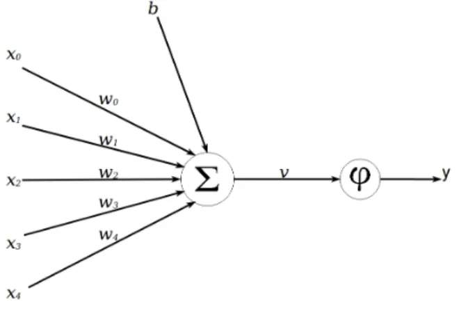
introduced in 1943 by Warren McCulloch and Walter Pitts [3], who created the first computational model of a neuron. The McCulloch-Pitts model of a neuron was ex-tended by Frank Rosenblatt in 1958 [4] to create the perceptron, which is the model commonly used in neural networks today. Figure 2.2 illustrates the perceptron model of a neuron. Inputs to the neuron are each multiplied by a weight, and the sum of these weighted inputs, along with a bias, is passed through an activation function. Equations 2.8 and 2.9 provide a mathematical definition of the perceptron.

Figure 2.2: Perceptron model of a neuron

vk = N−1 X i=0 wkixi+b (2.8) yk=φ(vk) (2.9)

Equation 2.9 is the process of applying a activation function to the output of 2.8. The purpose of the activation function is to apply a non-linearity to the neuron, which is what allows neural networks to learn complex non-linear functions. If the activation function was linear, the neural network would simply be a linear function approximator. The biological analog of the activation function would be to determine if a neuron is firing or not. Some of the most common activation functions include the Heaviside step, sigmoid, tanh, and relu (rectified linear unit) functions.

(22)

The most common type of neural network is a fully connected feed forward neural network. In this type of network, layers of perceptrons are constructed where the input to each neuron is output of all the neurons in the previous layer. These networks have an input and output layer, and any number of hidden layers. The term ”deep” used to describe neural networks refers to networks which have multiple hidden layers. Deeper networks are generally capable of a higher level of abstraction from the data. In all neural networks, information is stored in the weighted connections between neurons and the weights are determined through a training process.

2.2.1 Training

Neural networks are typically trained through a process called back-propagation, which aims to minimize a some loss function, often defined as the square difference between actual and desired output of the network. The derivative of this function with respect to the weights of the network can be interpreted as the gradient of the high dimensional surface created by the weights of the network. The weights can be updated by performing gradient descent, achieved by propagating calculated gradients backwards through the network. Theoretically there is a global minima that corresponds to the optimal set of weights that would minimize the loss function, but in practice gradient descent is only guaranteed to find a local minima. Many algorithms exist to best estimate the gradient and perform gradient descent such that a good minima is found.

2.2.2 Convolutional Neural Networks

Convolutional neural networks (CNN) are a special type of deep neural network that can perform high level abstractions of image data. CNNs were popularized by Yann LeCunn in 1998 with LeNet, an early successful application of CNNs to

(23)

handwritten and machine generated character recognition [5]. In a traditional pattern recognition process, features to be extracted from the image would be hand-crafted and a separate classifier would be trained to classify those features. The issue with this is the system is limited by the ability of the engineer to select the best features. In contrast, convolutional neural networks enable end-to-end learning where feature extraction and classification are trained together. This allows the best features from the image to be determined autonomously during training, and have led CNNs to become the state of the art on pattern recognition benchmarks.

There are several types of layers in a convolutional network: convolutional, pool-ing, and fully connected layers. The primary innovation is the convolutional layer. Convolutional layers are three dimensional, with a width, height, and depth. The width and height are the dimensions of the filters for that layer, and the depth refers to the number of filters in that layer. Neurons in convolution layers are connected to only a small region of the layer before it. This region is called the receptive field of the neuron and is the size of the filters. The filters are convolved with input im-ages to perform feature extraction, thus the values in the filter kernals are what are learned during training. Since neurons in the network are only connected to a small region in the image and because each region shares the same filter weights, there are few fewer parameters to learn in a CNN compared to a deep fully connected neural network. For the same reason, it is easy to parallelize the convolution operation in implementation. The popularity and success CNN’s has skyrocketed since the recent availability of powerful GPUs enables efficient parallel computation. After the convo-lutional layers of a network, the output is typically flattened into one large layer that is then input to several fully connected layers. These layers are intended to perform classification on the learned features from the CNN part of the network. LeNet [5] is a good example of how a simple CNN can be constructed for classification. CNNs are trained with same process of back-propagation mentioned in section 2.2.1.

(24)

2.3 Depth Sensing

The system designed in this thesis utilizes a depth camera to acquire depth images. The camera is modeled as a single point in 3d space, and each pixel in the depth image is the length of the ray extending from the center of the camera through that pixel until it collides with an obstacle. This provides a data dense representation of the environment that is particularly useful for determining where obstacles are in physical relation to the camera.

As of 2019, there are several different types of depth cameras. One type are stereo cameras, which utilizes two cameras and accompanying stereo depth algorithms to mimic the binocular ability of animal eyes to determine depth. The other type of depth camera are infrared (IR) time of flight cameras, which measure distance by pulsing IR light measuring the time it takes for that pulse to return through each pixel, from which the distance can be computing using the speed of light. Similar are IR cameras which instead measure the phase shift of the returning light, which can be used to determine distance.

The benefit of using depth cameras is that they provide a data dense representation of the world in 3-dimensions. Such information can be used to avoid obstacles low to the ground or above that would clip the top of the robot. Additionally, depth cameras that utilize infrared light are more invariant to lighting than regular RGB cameras, allowing them to work in a variety of lighting conditions such as outside or in dark rooms.

(25)

Chapter 3 RELATED WORK

The reinforcement learning system proposed in this paper was built upon the re-search of many others. This section provides an overview of the seminal rere-search that led to the decisions made in the design of the system proposed in this thesis. Ad-ditionally, the methods behind the conventional approach to the navigation problem are introduced.

3.1 Conventional Navigation

The navigation problem is typically solved using standard framework consisting of three main components: mapping, localization, and path planning. Mapping and localization addresses the problem of understanding where the robot is and what surrounds it, and path planning determines how to get from point A to point B.

3.1.1 SLAM

Simultaneous localization and mapping (SLAM) refers to the problem of having a robot build a map of an unknown environment, while at the same time knowing where it is within that map. This ability is often viewed as one of the core competencies for truly autonomous robots, and it is becoming increasing important with the emergence of robotics applications where autonomous motion planning is required, and GPS is not readily available or not accurate enough. With a known and up-to-date map, a robot has the information is needs to succesfully navigate its environment. Foun-dational approaches to SLAM are formulated as probabalistic posteriori estimation problems, where the two key solutions are through the application of the extended

(26)

Kalman filter and Rao-Blackwellized particle filters [6]. More modern approaches are based on iterative nonlinear optimization [7]. Sensors commonly utilized in the mapping and localization process include: LIDAR, RGB cameras, stereo cameras, IMUs, and wheel encoders. Although the SLAM problem has been solved theoreti-cally, SLAM algorithms face practical implementation challenges as robots move into challenging dynamic environments with lower-cost sensors.

3.1.2 Path Planning

The objective of path planning is to obtain an optimal or near optimal collision free path from a starting position to a goal position, within some constaints. These constraints could include: time, path length, proximity to obstacles, robot kinematics, and more. These methods require an map of the robot’s environment.

One widely applied path finding algorithm is A* [8]. A* is a best-first search algorithm that is formulated for weighted graph based problems. For many robotics problems, the weighted graph is a grid that is overlaid on top of an ocupancy map of the environement being navigated, where the weights are the cost of traversing that space. A* seeks to find the minimum cost path between the start and goal node of the graph, where the cost is the sum of the transition between nodes and a heuristic that estimates the cost of the cheapest path to get to the goal position. A* has been proven to find optimal paths. A downside of A* is that it cannot directly take into account the non-holonomic constraints of most robots; paths generated by A* must be smoothed to satisfy these constraints. A* has been adapted to find any-angle paths [9], and paths in dynamic environments [10].

Another popular type of path planning algorithms are sampling based algorithms. These methods randomly sample the configuration space of the robot, which for 2d navigation is the set of all possible positions and orientations of the robot. One such

(27)

sampling algorithm is probabilistic roadmaps, which connects random samples from the configuration space into a graph, which is then used to construct a path [11]. This method is probabilistically complete, meaning a path will always be found if it exists, but the path will need to be smoothed in order to achieve a physcially traversible path. Another algorithm is rapidly exploring random trees (RRT), which samples the configuration space to build random trees extending away from the starting position until the goal position is met [12]. The points can be sampled from the configuration space such that the potential path is always kinematically traversible by the robot. RRT is well adapted to high-dimensional, non-hononomic path planning problems. RRT* is an improved version of RRT that includes proven asymptotic optimality given infinite samples [13].

3.2 Reinforcement Learning

Reinforcement learning, introduced in section 2.1, is another method of deter-mining robot navigation controls. In contrast to the conventional approaches, these approaches model navigation as a Markov Decision process which can then be solved with a variety of reinforcement learning algorithms. This section outlines the key deep Q-learning algorithm, and the accompanying innovations of double Q-learning and dueling Q-networks that form the D3QN algorithm. The primary work of D3QN applied to obstacle avoidance that this thesis directly extends is introduced, and fi-nally some additional reinforcement learning algorithms applied to navigation are discussed.

3.2.1 Deep Q-Learning

Mnih, Kavukcuoglu, Silver et. al [14] applied deep neural networks to Q-learning to create deep Q-networks (DQN). The DQN algorithm was evaluated on 49 Atari

(28)

games, where the only information available to the algorithm are four 80x80 pixels images from the game screen and the current score of the game. DQN was found to outperform the previous state of the art reinforcement learning algorithms on 43 of the games, and was found to perform at 75% and above performance compared to a human professional player on 29 out of 49 games. The same algorithm with the same architecture and hyperparemeters was able to perform strongly across most games, despite some of the games varying significantly in play style.

DQN leverages several key innovations to achieve super-human results. The first key innovation of DQN was to apply deep convolutional neural networks. The net-work takes as input the current and three previous frames from the Atari game and outputs a Q-value for each of the potential joystick actions. Secondly, DQN utilizes an experience replay buffer. During training, the N previous transition ex-periences et = (st, at, rt, st+1) are stored in data base Dt = e1, ...., et. Batch updates for training the Q network occur at every time-step and are uniformly sampled from D, (s, a, r, s0) ∼ U(D). Experience replay smooths out learning, reduces learning variance, prevent oscillations, and helps prevent bias. The final key innovation was to use delayed and fixed version of the Q-network for target estimation to prevent oscillations in the data.

DQN uses the mean-squared error of the value estimates to determine Q-function updates.This reflected in the following loss Q-function for update iteration i: Li(θi) =E(s,a,r,s0₎_∼ _U₍_D₎[(YQ i −Q(s, a;θi))2] (3.1) Y_iQ =r+γmax a0 Q(s 0_{, a}0_;_θ− i ) (3.2)

The derivative of this loss function with respect to the weights θi gives the gradient used to perform backpropagation to update Q(s, a;θi). DQN uses a delayed and fixed version of the primaryQ(s, a;θi) network to produce target updateQ(s0, a0;θi−).

(29)

The target network parameters θ− are updated to be equal to the primary network parametersθ everyC iterations. When not using a target network, the same network is used to produce the targetY_iDQN and Q(s, a;θ). Updates to the network can move the target such that the Q-function is always chasing a target and never converging. Using a target network helps to prevent these oscillations.

Figure 3.1: Original Deep Q-Network proposed in [14]

Figure 3.1 illustrates the architecture of the deep Q-network applied to Atari games. The activation function of each layer is a ReLU activation function, with the exception of the activation of the last layer, which is a linear function. The number of neurons in the last layer is the same as the number of actions that can be taken for the particular Atari game being played. Having the network output a Q-value for each action is another innovation of the DQN algorithm, which is crucial as it allows all Q-values to be approximated from a single forward pass through the network, in contrast to a Q-network that takes as input a state and a potential action and outputs a single Q-value for that action. Approximating all Q-values from a single forward pass allows the algorithm to be much more efficient.

3.2.2 Double Q-Learning

The basic Q-learning algorithm introduced in background section 2.1.2 tends to overestimate action-value estimates, meaning that certain actions are learned to be

(30)

more valuable than they actually are. When the value of an action is overestimated, Q-learning learns to take that action the next time it’s in that state. This has the affect of preventing the optimal policy from being learned. Hasselt et. al. [15] demon-strated the impact of these action-value overestimations on DQN performance with Atari games and developed the double Q-learning algorithm to reduce the effects. Double Q-learning applied to DQN is referred to as DDQN, which was shown to con-sistently improve performance of DQN on most Atari games. The overestimation of Q-values can be attributed to the maximization of estimated action values when ap-proximating the optimal policy. The maximum valued action maxaQ(st+1, a) is used

for both estimating the optimal Q-value and for selecting the best action when follow-ing an -greedy policy. Separating maxaQ(s, a;θi) into Q(s0,argmaxaQ(s, a;θi), θi) in equation 3.3 illustrates how the maximum Q-valued action that is selected is also used for estimating the new Q-value. Both action selection and Q-value estimation are performed with the same neural network parameters θ.

Y_iQ =r+γmax a Q(s, a;θi) = r+γQ(s 0 ,argmax a Q(s, a;θi), θi) (3.3) Double Q-learning serves to prevent action-value overestimations by separating action selection and action-value evaluation. It can be implemented by selecting the actionawith weightsθaccording to a greedy policy, and evaluating that action for the target update with a different set of weights θ−, eq 3.4. Double-DQN has the target 3.4, the weights θ− are from the target network from [14]. Using the target network as the action-value evaluation network prevents needing three separate networks and provides the benefits of using a target network and of double Q-learning. Hasselt et. al. [15] evaluated the double DQN algorithm on the same set of Atari games as DQN in [14] and shows that in general, double Q-learning improves performance by reducing action-value overestimations.

Y_iDoubleQ=r+γQ(s0,argmax0 a

(31)

3.2.3 Dueling Q-Networks

Dueling Q-networks were introduced by Z. Wang, T. Schaul, M. Hessel, H. Has-selt, M. Lanctot, and N. Freitas, [16] with the intuition that performance will be improved if the agent can learn which states are valuable to be in without having to experience taking all possible actions in that state. This allows the Q-network to bet-ter identify the correct action when some of the possible actions are redundant. The neural network in dueling Q-network is identical to the DQN network proposed in section 3.2.1, however the fully connected layers splits into two separate streams, see figure 3.2. One stream estimates the value V(s) and the other stream estimates the advantage of taking a particular action in that stateA(s, a). The outputted Q-values actions is then represented by their sum

Qπ(s, a) =Vπ(s) +Aπ(s, a) (3.5)

Figure 3.2: Dueling Q-network Architecture [16]

The dueling Q-network architecture can be swapped out for the standard DQN architecture with all other aspects of the algorithm kept the same. The dueling architecture innovation, coupled with DDQN, improved the highest score achieved on 75% of the Atari games when compared to DDQN. The deep, double, and dueling innovations applied to Q-learning produces the D3QN algorithm applied in this thesis.

(32)

3.2.4 D3QN for Obstacle Avoidance

The D3QN algorithm was applied by L. Xie, S. Wang, A. Markham, and N. Trigoni in [17] to develop an obstacle avoiding agent for a differential drive robot. In contrast to DQN for Atari, where the state consists of four consecutive frames taken from an emulator, in this work the state consists of four consecutive 160x128 depth images. This state representation was selected to enable the agent to understand its position and velocity in relation to the obstacles in its environment. The action space consisted of seven different actions, two linear velocities v (0.2, 0.4 m/s) and five angular velocities ω (π 6, π 12, 0, − π 12 − π

6 rad/s). The agent selects one of these seven

actions at each timestep, producing ten unique behaviors. The reward function

r =        vcos(ω)δt−0.01 no collision −10 collision (3.6)

encouraged the robot to drive straight forward as fast as possible while avoiding colli-sions with obstacle. Upon collision with an obstacle, the robot receieves a−10 reward as a punishment for crashing. L. Xie, S. Wang, A. Markham, and N. Trigoni showed that this agent could be trained in simulation in simple and complex environments, and successfully deployed on a physical robot. Additionally, D3QN outperformed DDQN and DQN on the same obstacle avoidance tasks, suggesting that D3QN is well suited to for performing obstacle avoidance. This thesis primarily extends on this work to enable the same robot to both avoid obstacles and navigate to a desired goal location.

3.2.5 Alternative Algorithms

Reinforcement learning has been applied to robot navigation several other works. J. Zhang, J. T. Springenberg, J. Boedecker, and W. Burgard [18] applied DQN to

(33)

robot navigation from depth images where the robot can take one of four actions: stand still, turn left 90◦, turn right 90◦, and move forward 1 meter. They show that their reinforcement learning agent is able to train in one environment and success-fully generalize to another. G. Kahn, A. Villaflor, B. Ding, P. Abbeel, and S. Levine [19] applied model-free and model-based reinforcement learning into an generalized computation graph, and was able to have a RC car learn obstacle avoidance poli-cies directly from low resolution grayscale images. J. Zhang, J. T. Springenberg, J. Boedecker, and W. Burgard [18] applied a reinforcement learning algorithm called A3C to robot navigation from depth images and goal heading. With this approach, they achieved 70-85% success rates traversing unknown terrain.

(34)

Chapter 4 DESIGN

This chapter outlines the design of the proposed reinforcement learning agent. The motivation behind using depth images and a direction toward the goal is explained, the action space of the robot, and the the two neural network architectures used to approximate the Q-function of this reinforcement learning problem are introduced and analyzed.

A high level overview of the proposed reinforcement learning agent is presented in figure 4.1. The proposed system outputs suitable collision free velocities for a robot at 5 Hz

Figure 4.1: System overview

4.1 State Representation

At each time-step the agent uses the current state to decide what action to take to maximize future rewards. The state needs to contain enough information about the environment such that the agent is able to make the optimal decision. The state was selected to be a sequence of the current and three previous depth images captured from a depth camera, along with an angle θ representing the heading toward the desired goal.

(35)

4.1.1 Depth Images

Depth images provide crucial geometric information about the surroundings of a robot. A single depth image contains dense information about the proximity of obstacles in three dimensions, within the limits of the sensing depth camera. This dense representation of the environment provides a wealth of geometric information that would otherwise not be available through a 2-dimensional sensor such as LIDAR, or directly through RGB images captured by a standard camera. RGB images are also more variant to lighting, and contain color and texture information from which the proximity of obstacles is not immediately available without complex algorithms to infer depth. In contrast, depth images directly provide the depth information necessary for obstacle avoidance.

In addition to providing the agent with a dense representation of the immediate environment, using a sequence of current and previously captured depth images en-ables the agent understand the dynamics of its environment. The agent can infer the robot’s linear and angular velocity from the differences between images, along with the motion of dynamic obstacles in the environment. This mimics human un-derstanding of depth in that humans’ don’t continually calculate their exact velocity, but still understand their velocity by observing the world moving around them. Fig-ure 4.2 illustrates an example of a stack of four depth images taken while the agent is following a random policy. From these images it is possible to observe that the robot is moving forward, turned left, and then turned right.

(36)

(a)t= 0 (b) t= 1 (c) t= 2 (d)t= 3 Figure 4.2: Example stack of four 160x128 depth images taken following random policy, where t= 3 is the current depth image

4.1.2 Goal Heading

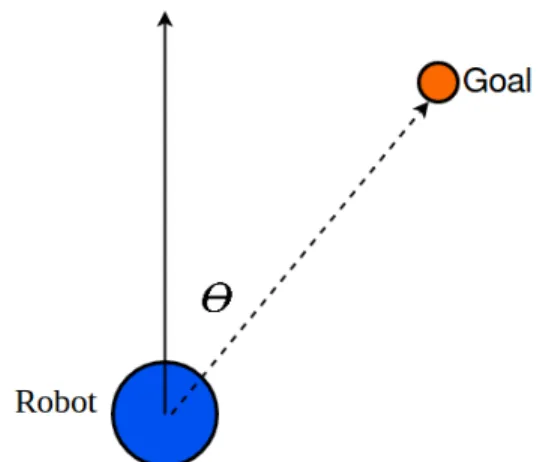
In addition to the depth images as part of the state, the agent also needs informa-tion that will enable it to approach the desired goal locainforma-tion. A very practical metric for this is the heading toward the goal location. In contrast to using the distance to the goal, which is difficult to sense in practice, measuring the relative heading does not does not have any dependence on mapping or localization. A good example is a robot approaching a visual objective while traversing through an unexplored cluttered space. The robot does not know where it is relative to its goal, and the goal position or object is far outside the maximum range of the sensing depth camera. The direc-tion to the goal could be easily determined, however, through detecdirec-tion with an RGB camera. The motive for this piece of information is drawn from how humans navigate. In general, humans don’t know the exact relative distance of their target location but do know what direction to go in that will get them closer to their objective. Includ-ing the relative headInclud-ing toward the goal location as part of the state eliminates the dependency on needing to know the exact relative distance to the goal. The relative heading provides critical information that the reinforcement learning agent needs to decide what actions to take to approach the goal. Figure 4.3 shows the robot heading and the angle θ to the goal.

(37)

Figure 4.3: Robot Heading and Goal

4.2 Action Space

The action space is dependent on the robot used and it’s physical limitations. In this thesis, the agent determines control actions for a robot commonly used in research called Turtlebot, a differential drive robot that is further discussed in section 5.2. For Turtlebot it is possible to command linear and angular velocity, so the action space was chosen such that the agent has control of seven unique linear and angular velocity commands. The linear velocities that the agent can select from are {0.2,0.4}m

sand the angular velocities that the agent can select from are {π

4, π 8,0,− π 8,− π 4} rad s . These specific velocities were selected because they allow the agent to move at safe speeds but also rotate quickly if necessary to avoid obstacles. The robot is restricted to only forward movement as it does not have a re-facing sensor that would allow it perform obstacle avoidance while driving in reverse. At each time step, the agent selects one action from this set of seven actions, meaning the agent can only change its linear or angular velocity, but not both in the same time step. This is important because it allows the action space to be as small as possible while still allowing a sufficient resolution of control. The size of the Markov Decision Process describing the reinforcement learning problem increases exponentially with the number of actions

(38)

that can be taken in each state, so choosing a smaller number of actions results in a Q-function that is easier to approximate.

4.3 Reward Function

The objective of the agent is reflected in the design of the reward function. For the problem of autonomous mobile robot navigation, the reward function should reward the agent for moving the robot toward and reaching the goal location, and penalize it for moving away from the goal and colliding with obstacles. To achieve this, the following reward function was designed:

r =                1 d <0.5 −1 collision v cos(θ)−0.01 otherwise (4.1)

If the distanced between the robot and the goal is less than 0.5 meters, the agent receives a reward of 1. A collision is considered if robot detects an object closer than 5 cm, and the agent receives a reward of−1. At all other time steps, the agent receives a reward ofvcos(θ)−0.01, wherev is the linear velocity of the robot,θ is the heading to the goal, and the constant −0.01 term serves to incentivize the robot to move toward the goal as fast as possible. This reward function shares some similarities to the reward function in section 3.2.4 used by L. Xie, S. Wang, A. Markham, and N. Trigon [17] who showed that it could be effectively used for obstacle avoidance. The reward function was modified to not only encourage the robot to not crash, but also move in the direction θ toward the goal location.

The scale of rewards was specifically chosen to be within the range [−1,1]. Fol-lowing the above reward function, the maximum reward the agent can receive on any non-terminal timestep is in the range [−0.07,0.05]. This makes the scale of the

(39)

re-wards for crashing and reaching the goal one to two orders of magnitude higher. This ensures that the agent learns that those experiences are very important in comparison to the other rewards.

4.4 Architectures

The neural network used to approximate the Q-function is a modification of the D3QN double dueling network introduced in [16] for playing Atari games and applied to obstacle avoidance in [17]. Since D3QN was already proven to work for obsta-cle avoidace, it shows promise for developing navigation agents for several reasons. Firstly, deep Q-learning [14] coupled with double Q-learning [15] provides a method for learning control policies directly from high dimensional inputs. Second, the in-novation of estimating state values and action advantages separately with dueling networks allows the function to be learned quicker [16]. Applying dueling Q-networks intuitively means that the agent can better estimate the value of taking actiona (changing linear or angular velocity to move toward a goal) without actually exploring those actions. The D3QN architecture as originally applied to Atari games can be seen in figure 4.4.

Figure 4.4: D3QN architecture for playing Atari games.

(40)

ar-chitectures to incorporate the critical heading information of the state, which informs the agent of what direction to drive. Other than modifying the architecture to include this new state information, the hyper-parameters of the architecture remain the same with the exception of size of the filters in the first convolutional layer being changed to 10x14, as introduced by [17] for obstacle avoidance. Both of these architectures are analyzed for 160x124 and 80x64 resolution images. The only change between these architectures for these resolutions is the size of the images after each convolutional layer, and the number nodes after the CNN output is flattened and connected to the fully connected layers of the dueling network. These two architectures, along with their parameters, are presented below.

4.4.1 D3QN-I

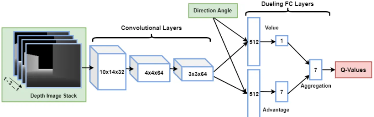
The first modification of D3QN, called D3QN-I, incorporates the direction angle as an additional image input to the neural network. This image has the normalized direction angle [−π, π]→[0,1] as the value for each pixel. This is inspired by AlphaGo [20], a reinforcement learning agent that outperforms top human players at the board game Go. State information on which player’s turn it was provided to the agent by replicating this binary value as the pixels of an image. This was passed into their convolutional neural network, along with the current and prior stone locations. Passing the direction angle into the convolutional neural network, along with the depth images, intuitively leads to features abstracted from the depth images that include some value determined by the angle to the goal. From these features, the dueling part of the architecture can then appropriately estimate the value of each possible action.

The architecture is illustrated in figure 4.5 and its parameters are outlined below in table 4.1 for full resolution (160x128) and half resolution (80x64) images. The

(41)

activation function of each layer is a ReLU activation function, with the exception of the output layer which is a special aggregation layer to sum action advantages and state value estimations. Note that when half resolution images are used as inputs, the resulting model has 74.83% fewer parameters than the model when full resolution images are inputted.

Figure 4.5: D3QN-I architecture

Table 4.1: D3QN-I Parameters Layer Size Stride Full Resolution # Parameters Half Resolution # Parameters Conv 1 10x14x32 8 4,512 4,512 Conv 2 4x4x64 2 1,088 1,088 Conv 3 3x3x64 1 640 640 FC Value 1 512 - 2,621,952 655,872 FC Advantage 1 512 - 2,621,952 655,872 FC Value 2 1 - 513 513 FC Advantage 2 8 - 4,104 4,104 total - - 5,254,761 1,322,601

(42)

4.4.2 D3QN-S

The second modifcation of D3QN, called D3QN-S, introduces the direction angle state information as an input the fully connected layers of the network. Intuitively, the state information is associated with the features abstracted from the convolutional layers of the network, which has already been shown to be effective at abstracting features for obstacle detection [17]. This is in contrast to the first architecture, where direction state information is instead associated with the depth images by the convo-lutional layers. The second architecture is illustrated in figure 4.6 and its parameters are outlined in table 4.2. This second network has 1024 total parameters more than the first model, since the the directional input is introduced into the two 512 fully connected layers. The activation function for all layers is a ReLU activation function, with the exception of the last layer being a special aggregation layer to sum action advantages and the state value estimation.

(43)

Table 4.2: D3QN-S Parameters Layer Size Stride Full Resolution

# Parameters Half Resolution # Parameters Conv 1 10x14x32 8 4,512 4,512 Conv 2 4x4x64 2 1,088 1,088 Conv 3 3x3x64 1 640 640 FC Value 1 512 - 2,622,464 656,384 FC Advantage 1 512 - 2,622,464 656,384 FC Value 2 1 - 513 513 FC Advantage 2 8 - 4,104 4,104 total - - 5,255,785 1,323,625

(44)

4.5 Deep Q-learning Algorithm Pseudo-Code

The algorithm applied to traing the approximating neural networks is outlined in the following pseudo-code:

Algorithm 2 Deep Q-learning with Experience Replay Pseudo-Code Initialize replay memory D to capacityN

Initialize dueling Q-network with random weightsθ Initialize target dueling Q-network with weightsθ− =θ for episode = 1, M do

t= 0

while st is not terminal do

With probability select a random actionat otherwise select at= argmaxaQ(st, a;θ)

Execute actionat and observert and state st+1

Store transition (st, at, rt, st+1) in D

Sample random minibatch of transitions (sj, aj, rj, sj+1) from D

if sj+1 is terminal then

yj =rj else

yj =rj+γQ(sj+1,argmaxa0Q(s_j₊₁, a0;θ);θ−) end if

Perform gradient descent on_E(sj,aj,rj,sj+1)∼ U(D)[(yj−Q(sj, aj;θ))

2_]_{w.r.t. θ} st←st+1 t←t+ 1 θ− ←θ every C steps end while end for

(45)

Chapter 5 IMPLEMENTATION

This chapter outlines the details of implementing the design presented in chapter 4, along with how the agent was trained and evaluated. Due to the large training time and amount of data required for the approximating Q-network to converge to a decent minima, it is impractical to fully train the agent on a real robot. Additionally, training on real robot would require constant human supervision to reset the robot upon crashing or reaching the goal position. The agent is instead trained in a simulator. The major benefits of training in a simulator include being able to speed up simulation multiple factors of real-time, and being able to script training such that training is consistent and can automatically reset when the agent reaches terminal states. For these reasons, the agent proposed in this thesis is implemented, trained, and evaluated entirely in simulation.

5.1 Simulator and ROS

Training the reinforcement learning agent proposed in this thesis requires a simu-lator that must be able to: simulate faster than real-time, simulate depth cameras to produce depth images for training, support a wide variety of obstacles, and must be a full physics simulator to accurately simulate robot dynamics. The simulator that best supports the requirements for training the navigation agent is an open source simulator called Gazebo. Gazebo provides physics simulation and sensors simulation at faster than real-time, the ability to construct worlds to simulate in, models of commonly used research robots, and easy integration with an open source robotics software framework called the Robot Operating System.

(46)

The Robot Operating System (ROS) is a flexible robotics software framework that provides many of the tools and open source software necessary to build complex robotic systems. ROS provides a communication graph that allows robotics software, such as low level firmware, control algorithms, visual perception algorithms, navi-gation algorithms, etc. to be designed and connected in an organized and modular fashion. It also provides implementations of common fundamental robotics algorithms so that robotics development speed can be greatly increased from all algorithms not needed to be developed in-house. ROS can interface directly with Gazebo, without necessitating any changes to software in order to run in simulation as opposed to the real world, and ROS systems can run directly on a clock provided by Gazebo, which allows the entire robotics software system to run exactly as it would in real-time but accelerated to the desired speed of the simulation. The particular distribution of ROS used is ROS Kinetic Kame. ROS and Gazebo provide the necessary tools for training reinforcement learning agents.

5.2 Turtlebot Robot

Turtlebot is robot commonly used in robotics research. It features a two-wheeled differential drive train and a Microsoft Kinect sensor for depth sensing. The differen-tial drive train allows the robot to turn about its center point, which is very useful for changing directions without needing to move forward or backward. Figure 5.1b shows the two wheeled differential drive train of the turtlebot. It is supported by casters to prevent the robot from tipping due to having only two wheels. The maximum linear velocity of the Turtlebot is 0.65m_s, so the action space of the reinforcement learning agent is designed such that the maximum velocity the agent can decide to go is 0.4m_s, safely within the Turtlebot’s ability. The motivation behind the design of the action space is discussed in section 4.2.

(47)

The Kinect depth sensor on the Turtlebot can be seen in figure 5.6a. A Kinect consists of an RGB camera, a depth sensor, and a microphone array, and was origi-nally developed for gaming applications. The Kinect quickly caught on for robotics applications however, as the included depth sensor can produce with 640x480 depth images at up to 30 Hz, with a range of 0.4 meters to 4.5 meters.

(a) View of Kinect sensor (b) Bottom view of differential drive train

Figure 5.1: Turtlebot Model

Turtlebot is open source and a model is publicly available for the Gazebo simu-lator. This model behaves in simulation just as a Turtlebot in the real world would, with accurate physics and dynamics simulation. The Kinect sensor is modeled ideally and produces 640x480 ideal depth images at 20Hz with no noise and range clipped exactly in the range 0.05 meters to 5 meters. The close range is used purely in sim-ulation for determining collisions, and the range is further clipped to 0.4 meters to realistically model an actual Kinect. In real world implementation, an extra sens-ing technology such as low cost sonar would need to be employed to determine close range collisions for training on real hardware purposes. The captured depth images are resized to be input to the Q-network.

(48)

5.3 Training

The agent is trained in a simple and a complex environment. The training of the agent is broken up into episodes, where an episode begins with a start and goal location for the robot being selected from a hand designed set of positions. Each environment has an 5 start and 14 goal locations, which gives 70 unique paths for the robot to traverse, which should lead to agents generalizing to paths instead of overfitting to a select few number of paths. During the episode the agent receives feedback from the environment in the form of depth images and direction to the goal, and it determines the action it needs to take to move toward the goal. The episode concludes when the agent crashes into an obstacle or reaches its goal location within a 0.5 meter radius. There are no constraints on the orientation of the robot once it reaches the goal location, it just needs to be within the specified distance. A collision is considered when any depth image pixel value is less than 0.4 meters. or when bumpers on the Turtlebot are triggered by bumping into an object.

The training was experimentally determined for all models to take at least 400,000 timesteps to converge, where a timestep is 0.2 seconds. From this, a single training can be calculated to take at least 22.2 simulation hours. Most models and hyper-parameter changes were trained three times to obtain an average of learning that better indicates performance. Training three times leads to each test taking at least 67 simulation hours, which is almost three days of training just to evaluate one model with a particular set of hyper-parameters.

Training was conducted on several different machines. One machine is a laptop with a Intel core i7 processor, an NVIDIA GTX-860M GPU with 2GB VRAM, and 8GB of RAM. The other machine is a desktop computer with an AMD FX-4100 Quad-Core processor, an NVIDIA GTX-1050 GPU with 4GB VRAM, and 8 GB RAM. The rest of the machines are g2.2xlarge GPU instances provided by Amazon

(49)

AWS. All machines run Ubuntu 16.04 as ROS and Gazebo are designed to run on Linux based systems. On these machines, the simulation can be sped up to a factor of three, depending on the model being trained. This is absolutely crucial as this algorithm would not be feasible to train, evaluate, and iteratively develop otherwise in any practical length of time.

Tensorflow, a Python machine learning library developed and supported by Google, was used to construct and train the neural networks used in this thesis. The imple-mentation of this work is built on the open source impleimple-mentation of D3QN and obstacle avoidance provided in [17]. The algorithm and software to interface with ROS and Gazebo was written in Python 2.7. The pseudo-code of the algorithm is specified in section 4.5. Each each training time-step, the agent accumulates a new experience for the experience replay buffer, and samples a minibatch of experiences from the buffer to train the network on. The buffer is rolling such that a fixed number of previous experiences are stored. The policy the agent follows is changing each time step during the episode.

5.3.1 Environments and Paths

The agent was trained in a simple and complex environment to best evaluate each model. Each environment is an area of 7x7 m2 _{enclosed by 2 meter high walls.}

During training, the agent encounters a variety of obstacles that it must navigate the robot around. Some of these obstacles, along with how they are sensed by the depth camera, are displayed in figure 5.2. These obstacles range from large simple blocks to small cans and are intended to expose the agent to the variety obstacles that it would potentially encounter if implemented on a real robot.

(50)

Figure 5.2: Example obstacles captured in depth images

The agent was first trained in a very simple environment of large blocks only to evaluate if the agent is at all capable of learning a collision free navigation policy. An agent trained in this environment should be able to travel through a clutter free building. Figure 5.3a shows an image of this simple environment. The start and goal locations can be seen in figure 5.3b. Starting locations are in the center and in the corners of the environment, while goal locations are distributed uniformly throughout the environment. This leads to the agent being exposed to 70 unique paths with varying lengths, with the average path length being 8.13 meters.

(51)

(a) Side View (b) Start and Goal Locations

Figure 5.3: Simple Training Environment

The complex environment was designed such that the agent learns how to navigate in cluttered spaces. Start and goal locations were selected in the same way as the simple environment, with start locations in the corners and center, and goal locations distributed uniformly throughout. Figure 5.4a shows this complex environment, and its start and goal locations are shown in figure 5.4b. The average path length in the complex environment is 8.64 meters.

(52)

5.3.2 Hyper-Parameters

The hyper-parameters of training were overall kept similar to the those used in the D3QN model applied to obstacle avoidance [17], with the exception of several parameters.

Table 5.1: Baseline Hyper-parameters

Hyper-Parameter Value

Gammaγ 0.99

Initial Epsilon 1

Final Epsilon 0.01

Exploration Steps 50,000

Experience Replay Buffer Size 50,000

Batch Size 8

Target Network Update Rate τ 0.001

Learning Rate 0.0001

Gammaγ is the discount factor for future rewards, introduced in equation 2.1. A higherγ means that rewards many time steps away are valued similarly to the current or near future rewards. In contrast, a low gamma results in the agent being near sighted and focusing primarily on short term rewards. For the problem of navigation, γ is selected to be a high value of 0.99 so that rewards far in the future, such as reaching the goal location to receive a large reward, are heavily taken into account.

Initial epsilon, final epsilon, and the number of exploration steps describe the -greedy algorithm adopted to encourage the agent to explore new actions and states. Recall from section 2.1.2 which introduces the problem of exploration vs. exploitation. To maximize reward, the agent must take the optimal action at each time-step in order

(53)

to follow the optimal policy. These optimal actions wont be learned, however, if many unique actions and states are not explored during training. One exploration strategy is to at each time step during training the agent take a random action with probability , which should sufficient explore the state and action spaces. In this implementation, is 1 at the beginning of training and linearly decays at each time step for 50,000 time steps, down to an of 0.01 where is remains until training concludes. This ensures the agent explores the state and action spaces sufficiently, and continues to occasionally explore to make small optimizations toward the optimal policy.

The experience replay buffer size was selected to be 50,000, with a batch size of 8. This means that at each timestep the agent trains on a mini-batch of 8 experiences sampled uniformly from the previous 50,000 experiences experienced by the agent.

Target network update rate τ which describes how frequently the target network should be updated to have the same weights as the online network. Aτ value of 0.001 results in the target network being updated every 1000 time steps.

The final parameter is the learning rate, which is used by the ADAM optimizer [21] to perform gradient descent. A standard value of 0.0001 was chosen.

5.4 Evaluation

After training, models are evaluated in several environments different from the training environments and compared based on how successfully they can navigate to goals. The overall distribution of actions taken is also observed during each evaluation in an effort to better understand the behavior of each model.

The evaluation environments contain the same obstacles as the training environ-ments but in different configurations. This tests each model on how well it generalizes to navigating, and ensures that each model hasn’t over-fit and memorized specific

(54)

paths from the training environment. Each environment is designed to have 5 unique starting and 20 unique goal locations, which results in the agent being tested on 100 unique paths. Below are images of the simple and complex evaluation environments, and their starting and goal positions.

Figure 5.5: Simple evaluation environment, average path length 8.18 me-ters

Figure 5.6: Complex evaluation environment, average path length 8.4 me-ters

(55)

Chapter 6 RESULTS

The objective is to train and evaluate the two proposed extensions of the D3QN model. Both architectures are trained and evaluated for 160x128 and 80x64 resolu-tion images, the motivaresolu-tion being that smaller models train faster and are therefore preferable if performance is the same regardless of resolution. Relevant metrics such as average reward per episode,the percentage of successful goals reached, and maxi-mum Q-value are presented to best understand how the models train and determine the training cutoff for the best performance. Each model is evaluated in both simple and complex evaluation environments that differ from the training environments, as introduced in 5.3.1 and 5.4, and relevant reward and success metrics are collected. This data is to ensure that the models have learned sufficient general behaviors. Fi-nally, an example state is fed forward through one of the trained models and its output Q-values are analyzed.

6.1 Training

Several metrics are collected during training. One metric is the average total sum of rewards received each episode. The total rewards each episode tends to be very noisy, as the maximum reward that can be received during each episode is dependent on the length of the randomly chosen path, and because small changes in the weights of the neural network during training can lead to large changes in the distribution of states that the agent visits [2]. The rewards were processed with a running average of 100 to obtain a cleaner curve representing learning progress.

(56)

by observing the average maximum Q-value outputted at each training step for a fixed number of states. This set of predetermined states is collected when following a random policy, In this implementation, 5 unique states are used for this average, an example of which can be seen in figure 6.7.

An average of the percentage of goals successfully reached is collected, and pro-cessed with a running average of 250. The reason behind this longer running average is because it is possible that many short paths could be randomly selected during training, so a long running average reduces this effect. This percentage success data indicates how well an agent actually succeeds at navigating the robot to the goal. In general, these curves resemble their average reward curves since reaching a goal results in a high reward of 1, which has a large impact on the reward curve.

Because the models are initialized with random weights, training differs slightly between each run. In an effort to reduce this variability and best understand how each model trains, most models were trained three times to obtain an average of the training data. Each individual training was run for at least 400,000 time steps, which is 22.2 hours of simulation training time. Some models were found to require substantially more training time than others.

6.1.1 Simple Environment

The two models and two resolutions were first trained in a simple environment. Below in figure 6.1a is a plot of the average total rewards received each episode. Figure 6.1b illustrates the average Q-values of each model learning in the simple environment.

(57)

(a) (b)

Figure 6.1: Simple environment training results