Digital Commons@Georgia Southern
Electronic Theses and Dissertations Graduate Studies, Jack N. Averitt College ofFall 2017
Application of the Misclassification Simulation
Extrapolation (Mc-Simex) Procedure to Log-Logistic
Accelerated Failure Time (Aft) Models In Survival
Analysis
Varadan Sevilimedu
Follow this and additional works at: https://digitalcommons.georgiasouthern.edu/etd
Part of the Epidemiology Commons, Health Services Research Commons, and the Other Public Health Commons
Recommended Citation
Sevilimedu, Varadan, "Application of the Misclassification Simulation Extrapolation (Mc-Simex) Procedure to Log-Logistic Accelerated Failure Time (Aft) Models In Survival Analysis" (2017). Electronic Theses and Dissertations. 1659.
https://digitalcommons.georgiasouthern.edu/etd/1659
This dissertation (open access) is brought to you for free and open access by the Graduate Studies, Jack N. Averitt College of at Digital Commons@Georgia Southern. It has been accepted for inclusion in Electronic Theses and Dissertations by an authorized administrator of Digital Commons@Georgia Southern. For more information, please contact [email protected].
(MC-SIMEX)PROCEDURETOLOG-LOGISTICACCELERATEDFAILURETIME(AFT) MODELSINSURVIVALANALYSIS
by
VaradanSevilimedu
UndertheDirectionofLiliYu
ABSTRACT
Survivalanalysisisthestudyoftimetoeventoutcomes. AcceleratedFailureTimemodels(AFT) serveasausefultoolinsurvivalanalysistostudythetimeofoccurrenceofaneventanditsrelation tothecovariatesofinterest. TheaccuracyofestimationofparametersinAFTmodelsisdependent uponthecorrectclassificationofbinarycovariates.Consideringthatperfectclassificationishighly unlikely,itisimperativethattheperformanceoftheexistingbias-correctionmethodsbeanalyzed inAFTmodels. However,certainareasofbias-correctioninAFTmodelsstillremainunexplored. One of these unexplored areas, is a situation where the survival times follow a log-logistic dis-tribution. In this dissertation, we evaluate the performance of the Misclassificationsimulation extrapolation (MC-SIMEX) procedure, a well known procedure for bias-correctiondue to mis-classification,inAFTmodelswherethesurvivaltimesfollowastandardlog-logisticdistribution. In addition, a modifiedv ersiono ft heM C-SIMEXp rocedurei sa lsop roposed,t hatp rovidesan advantageinsituationswherethesensitivityandspecificityofclassificationareun known.Lastly, theperformanceoftheoriginalMC-SIMEXprocedureinlungcancerdataprovidedbytheNorth CentralCancerTreatmentGroup(NCCTG),isalsoevaluated.
(MC-SIMEX)PROCEDURETOLOG-LOGISTICACCELERATEDFAILURETIME(AFT) MODELSINSURVIVALANALYSIS
by
VARADANSEVILIMEDU
MBBS.,GandhiMedicalCollege,India,2004 MPH.,GeorgiaSouthernUniversity,2010
ADissertationSubmittedtotheGraduateFacultyofGeorgiaSouthernUniversityinPartial FulfillmentoftheRequirementsfortheDegree
DOCTOROFPUBLICHEALTH STATESBORO,GEORGIA
VARADAN SEVILIMEDU All Rights Reserved
APPLICATIONOFTHEMISCLASSIFICATIONSIMULATIONEXTRAPOLATION (MC-SIMEX)PROCEDURETOLOG-LOGISTICACCELERATEDFAILURETIME(AFT)
MODELSINSURVIVALANALYSIS
by
VARADANSEVILIMEDU
Major Professor: Lili Yu
Committee: Hani M. Samawi Haresh Rochani
ElectronicVersionApproved: December2017
ACKNOWLEDGMENTS
I would like to thank Drs. Lili Yu, Hani Samawi and Haresh Rochani of the Department of Bio-statistics at the Jiann Ping Hsu College of Public Health, for providing their time and effort in making this dissertation a success.
TABLE OF CONTENTS Page ACKNOWLEDGEMENTS . . . 2 LIST OF TABLES . . . 5 LIST OF FIGURES . . . 7 CHAPTER 1 INTRODUCTION . . . 8 2 LITERATURE REVIEW . . . 11 Regression Calibration . . . 11 Pooled estimation . . . 12 Multiple imputation . . . 12
Corrected score function . . . 13
Estimated partial likelihood function . . . 13
Misclassification simulation extrapolation . . . 14
3 METHODOLOGY . . . 16
Accelerated failure time models (AFT) . . . 16
Basic notation and formula . . . 16
Specifications of AFT . . . 17
Likelihood function of AFT models . . . 18
Log-logistic AFT regression models . . . 20
An overview of log-logistic distribution . . . 20
Specifications of log-logistic AFT regression models . . . 21
An overview of the MC-SIMEX procedure . . . 22
The original MC-SIMEX procedure . . . 22
Modified MC-SIMEX procedure . . . 29
4 Simulation study . . . 32
Overview of the existing simulation method . . . 32
Overview of the proposed simulation method . . . 32
Data simulation and estimation of parameters . . . 36
Results of the performance of the original and modified MC-SIMEX estimator . 38 Results for a sensitivity of 80% and specificity of 80% . . . 38
Results for a sensitivity of 90% and specificity of 70% . . . 46
Robustness . . . 46
Conclusion . . . 53
5 Application to lung cancer data . . . 58
Introduction . . . 58
North Central Cancer Treatment group (NCCTG) - Lung cancer data . . . 59
Misclassification matrix . . . 59
Distribution of survival times . . . 60
Analysis . . . 61
Results . . . 62
6 Conclusion . . . 66
LIST OF TABLES
Page Table 4.1: Results of the MC-SIMEX procedure using log-logistic distribution of survival times. Sensitivity = 80%, Specificity = 80%. Trueβvalues areβ1 =−log2andβ2 = 0.5 . . . 40
Table 4.2: Results of the MC-SIMEX procedure using log-logistic distribution of survival times. Sensitivity = 80%, Specificity = 80%. Trueβvalues areβ1 =−log2andβ2 =−0.5 . . . 41
Table 4.3: Results of the MC-SIMEX procedure using log-logistic distribution of survival times. Sensitivity = 80%, Specificity = 80%. Trueβvalues areβ1 =log2andβ2 = 0.5 . . . 42
Table 4.4: Results of the MC-SIMEX procedure using log-logistic distribution of survival times. Sensitivity = 80%, Specificity = 80%. Trueβvalues areβ1 =log2andβ2 =−0.5 . . . 43
Table 4.5: Results of the modified MC-SIMEX procedure using log-logistic distribution of survival times. Sensitivity = 80%, Specificity = 80%. Trueβvalues areβ1 =−log2andβ2 = 0.5 . . . 44
Table 4.6: Results of the modified MC-SIMEX procedure using log-logistic distribution of survival times. Sensitivity = 80%, Specificity = 80%. Trueβvalues areβ1 =−log2andβ2 =−0.5 . . . 45
Table 4.7: Results of the MC-SIMEX procedure using log-logistic distribution of survival times. Sensitivity = 90%, Specificity = 70%. Trueβvalues areβ1 =−log2andβ2 = 0.5 . . . 47 Table 4.8: Results of the MC-SIMEX procedure using log-logistic distribution of survival times. Sensitivity = 90%, Specificity = 70%. Trueβvalues areβ1 =−log2andβ2 =−0.5 . . . 48
Table 4.9: Results of the MC-SIMEX procedure using log-logistic distribution of survival times. Sensitivity = 90%, Specificity = 70%. Trueβvalues areβ1 =log2andβ2 = 0.5 . . . 49
Table 4.10: Results of the MC-SIMEX procedure using log-logistic distribution of survival times. Sensitivity = 90%, Specificity = 70%. Trueβvalues areβ1 =log2andβ2 =−0.5 . . . 50
Table 4.11: Results of the modified MC-SIMEX procedure using log-logistic distribution of sur-vival times. Sensitivity = 90%, Specificity = 70%. Trueβvalues areβ1 =−log2andβ2 = 0.5 51
Table 4.12: Results of the modified MC-SIMEX procedure using log-logistic distribution of sur-vival times. Sensitivity = 90%, Specificity = 70%. Trueβvalues areβ1 =−log2
Table 4.13: Results of the MC-SIMEX procedure with the log-logistic distribution of survival times, but misspecified as a Weibull distribution. Sensitivity = 80%, Specificity = 80%. True β
values areβ1 =−log2andβ2 = 0.5. . . 54
Table 4.14: Results of the MC-SIMEX procedure with the log-logistic distribution of survival times, but misspecified as a Weibull distribution. Sensitivity = 80%, Specificity = 80%. True β
values areβ1 =−log2andβ2 =−0.5. . . 55 Table 4.15: Results of the MC-SIMEX procedure with the log-logistic distribution of survival times, but misspecified as a Weibull distribution. Sensitivity = 90%, Specificity = 70%. True β
values areβ1 =−log2andβ2 = 0.5. . . 56
Table 4.16: Results of the MC-SIMEX procedure with the log-logistic distribution of survival times, but misspecified as a Weibull distribution. Sensitivity = 90%, Specificity = 70%. True β
values areβ1 =−log2andβ2 =−0.5. . . 57
LIST OF FIGURES
Page Figure 1: PDF, QQ plot, PP plot and the CDF of empirical data compared to a log-normal distri-bution . . . 60 Figure 2: PDF, QQ plot, PP plot and the CDF of empirical data compared to a log-logistic distri-bution . . . 61 Figure 3: PDF, QQ plot, PP plot and the CDF of empirical data compared to a Weibull
distribution . . . 62 Figure 4: PDF, QQ plot, PP plot and the CDF of empirical data compared to a logistic
distribution . . . 63 Figure 5: Hazard functions associated with the lung cancer data considering the performance score category (PS) as the covariate. . . 64 Figure 6: Plot of the simex and naive estimators with their 95% confidence intervals. The x-axis represents the type of estimator and the y-axis represents theβˆvalues . . . 65
Chapter 1
INTRODUCTION
Survival analysis is the study of time-to-event outcomes, and is commonly used in mor-bidity and mortality analyses[1]. The accuracy of estimation of parameters in survival models depends upon the correct specification of binary covariates in the model. However, correct spec-ification of binary covariates seldom occurs, thus resulting in biased parameter estimates. For example, misclassification of immunization status resulted in biased hazard estimates of preterm birth, in a study by Ahrens et al. in 2012[2]. Misclassification of radiation exposure status resulted in biased hazard estimates in a study by Prentice in 1982[3, 4]. Misclassification of socioeconomic status resulted in biased estimates of risk of chronic disease, in a study by Kauhanen et al. in 2006[5, 6]. Despite the common occurrence of misclassification error, more research in this area is still needed.
Misclassification error can be classified into non-differential and differential misclas-sification error. Non-differential misclasmisclas-sification error occurs when the information provided by
W (misclassified or naive covariate), aboutY (response) is irrelevant as long as its corresponding true covariateXand the other confounding covariateZ are available. In this case,W is called the surrogate forX. For example, classifying an individual as hypertensive based on his/her systolic blood pressure measurement on a single day (W), versus systolic blood pressure measurement over a prolonged period of time (X) can result in non-differential misclassification error[7]. On the other hand, if W provides additional information about Y, even whenX and Z are already available, then a differential misclassification error ensues. For example, assigning an individual to a category of high risk for coronary heart disease, based upon total cholesterol measurements as opposed to low density lipoprotein (LDL) measurements, can result in differential misclassifica-tion error [8]. In this dissertamisclassifica-tion, we focus mainly on non-differential misclassificamisclassifica-tion error.
Survival analysis broadly employs two models: the cox regression model and the accel-erated failure time model (AFT). The Cox regression model regresses the risk/hazard of a certain event, at a certain time, on the risk/hazard at baseline and on the covariates included in the model. The AFT model, on the other hand regresses the log of the time of occurrence of an event on the covariates of interest[9, 10]. The effect of misclassification has been well studied in Cox regres-sion models[11]. Ahrens et al.[2] studied the effect of misclassification using the probabilistic bias analysis in a Cox regression model. Cole et al.[12] used the regression calibration and multiple im-putation approach to correct for the bias caused by misclassification in a Cox proportional hazards model. Zucker et al.[13] used the weighted least squares methods for correction of misclassifica-tion in a Cox propormisclassifica-tional hazards model, followed by the pseudo-partial likelihood[14] and the corrected score function approach[15, 16]. Bang et al.[17] apply the pooled estimation technique proposed by Spiegelman in 2001[18], to the Cox proportional hazards model. Zhou and Pepe[19] used an estimated partial likelihood function to correct for misclassification-bias in Cox regression models. However, the effect of misclassification has not been studied extensively in AFT mod-els, despite the transparent interpretation provided by them[20, 21]. Bang et al.[17] studied the effect of misclassification in survival data where the survival times follow the Weibull distribution. Slate et al.[22] studied the effect of misclassification in a log-normal AFT model. The Weibull and the log normal distributions can only model survival data where the hazard rate is monotonic. However, survival data in which the hazard rate does not follow a monotonic pattern, is also com-mon. For example, breast cancer and lung cancer [23, 24]. The log-logistic distribution is a very popular distribution to model such non-monotonic patterns[23]. Despite the importance of log-logistic distribution in survival studies[23], and its flexibility in accommodating non-monotonic hazards[23, 24], the effect of misclassification in log-logistic AFT models has not been explored yet. Therefore, in this dissertation, we study the effect of non-differential misclassification of bi-nary covariates in a log-logistic AFT model.
MC-SIMEX (Misclassification Simulation Extrapolation), is a simulation-based method that makes efficient use of misclassification rates (sensitivity and specificity) to produce bias-corrected mates. MC-SIMEX is a flexible approach which only requires the presence of a consistent esti-mator in the absence of misclassification error. In this dissertation, we employ the MC-SIMEX method to handle non-differential misclassification of binary covariates in a log-logistic AFT model. Further details of the MC-SIMEX procedure and the log-logistic AFT model are given in the Methodology section.
Chapter 2
LITERATURE REVIEW
In this chapter, we review the methods that have been used for the correction of bias caused by misclassification error in survival analysis. Over the period of the past three decades, several methods have been proposed and applied to correct for bias in parameter estimates caused by misclassification error.
2.1 Regression calibration
Regression calibration (RC) is a well known method used for correction of bias caused by measurement error[25, 26]. In this method, the value of the true covariate X is estimated by regressingX on the naive covariateW [27, 28]. The estimate thus obtained is then used as a sub-stitute forX in non-validation data[27]. The standard errors of these estimates are calculated by using statistical techniques such as bootstrapping or sandwich methods[27].
Even though the RC method is predominantly used for correction of measurement error in continuous covariates[29, 30], its convenience and ease of interpretation has led to its use, even in binary covariates that are prone to misclassification[17]. Cole et al.[12] studied the effect of mis-classification of categorized glomerular filtration rate (GFR) on the 4 year incidence of end stage renal disease (ESRD) using regression calibration in the Cox proportional hazards model. Bang et al.[17], used the regression calibration approach to correct for bias caused by misclassification, in a simulation study, where the survival times followed Weibull distribution.
The regression calibration method assumes that the RC model offers a good fit to the data and that the censoring mechanism involved is independent of the conditional distribution of
data and non-normal data[17, 31].
2.2 Pooled estimation
Spiegelmann[18] proposed the pooled estimation method to increase the efficiency of parameter estimates obtained through regression calibration. This method involves calculating the weighted averages of coefficients obtained, both from regression calibration and from primary re-gression in validation data. Bang et al.[17], applied the pooled estimation method to survival data, using the Cox regression model.
While the pooled estimation technique provides the advantage of improved efficiency, its performance is also contingent upon availability of large validation datasets. However, in the context of Cox regression models, the availability of large validation datasets is not always feasible[17].
2.3 Multiple Imputation (MI)
Multiple imputation was originally developed by Rubin et al.[32, 33], to correct for bias caused in parameter estimates, due to missing values in the true covariate. MI involves fitting a logistic regression model between the true covariate X and the naive covariate W, in the validation data i.e. logitP(X = 1|W). The naive covariate in the non-validation data is then replaced by the corrected value (0 or 1) by using the estimated probability from the logit function[17]. Cole et al.[17, 12], used the multiple imputation for measurement error (MIME) algorithm in the Cox proportional hazards model, assuming that data was missing at random (MAR)[33].
The advantage of using an MI procedure is that it uses the values of true covariates, whenever available[17]. In addition to this, it can handle differential measurement error better
than other methods[34, 35]. Finally, it is also very user-friendly and is easily available in any standard statistical package[17]. However, it has two disadvantages, one being that the correct specification of the model is crucial for its successful performance. The second disadvantage is that MI is harder to implement in data with censored outcomes[36, 37].
2.4 Corrected score function
Zucker et. al.[15, 16, 38], suggested a corrected score function approach, to correct for bias caused by misclassification of covariates in Cox regression. If the true score function in the ab-sence of misclassification is represented byΨtrue(Y, Z, X, θ), then the corrected score function in
the presence of misclassification of X can be represented asΨCS(Y, Z, W, θ), where the expected
value of the corrected score function equals the true score function[27]. This corrected score func-tion is then used for the estimafunc-tion of the parameter vectorθand the calculation of standard errors, using procedures such as the bootstrap method or the sandwich method[17]. Augustin[38, 39] proposes an exact corrected score estimate for the proportional hazards model in the presence of heteroscedastic measurement error.
The corrected score function can accommodate situations where the validation sample is not representative of all study participants[17]. Another distinct advantage of the corrected score function method is that it allows for dependence of the censoring mechanism on the true exposure variable X. However, there is loss of efficiency in estimating theΠmatrix, which is used for esti-mating the value of the true variableX fromW[17]. In addition, when the number of individuals at risk gets smaller as time progresses, numerical problems are known to occur in calculating the corrected score function[17, 40, 41].
Based on their previous work on uncensored data[42, 43], Zhou and Pepe[19] proposed an estimated partial likelihood for inference using information from both validation (X) and non-validation data (W). For non-validation data, they calculate the empirical risk function by averag-ing the values of risk functions for individuals in the validation data, that have the same covariate value. The total estimated risk function is the sum of risk functions over the validation dataset and the non-validation dataset. The relative risk parameter estimate is then obtained by maximizing the estimated partial likelihood function.
The estimated partial likelihood approach does not make assumptions regarding the baseline hazard function nor the conditional distribution ofX givenW, which is estimated non-parametrically. However, the disadvantage with this method is that when the dimension of W is large, the sample size for each substratum of W may be small, which may result in unstable esti-mates. A second disadvantage with the estimated partial likelihood method is that it assumes that the validation sample comes from a simple random sample, a non-adherence to which can result in unstable estimates[19].
2.6 Misclassification Simulation extrapolation (MC-SIMEX)
The Simulation extrapolation method (SIMEX) was first proposed by Cook and Stefanski[44] in 1994 to correct for bias caused by measurement error in continuous covariates. He et al.[45] first proposed the use of SIMEX method in survival analysis when continuous covariates were subject to measurement error, using data from the Busselton Health Study[46]. Kuchenhoff et al.[47, 44] in 2006 came up with a modification of the SIMEX procedure that could be applied to a situation where there is measurement error in binary/categorical variables. Since the measurement error in categorical variables is equivalent to misclassification, they called it the misclassification SIMEX or simply MC-SIMEX. Slate et al.[22] applied the MC-SIMEX procedure to evaluate the effect of misclassification in periodontal outcomes, in a log-normal AFT model. Bang et al.[17], in their
re-view, evaluate the MC-SIMEX procedure, by using a Poisson approximation[48, 49] to the Weibull AFT model. The details of the MC-SIMEX procedure are provided in the Methodology section.
Chapter 3
METHODOLOGY
The main purpose of this dissertation is to extend the works of Bang et al.[17] and Slate et al.[22] by applying the MC-SIMEX procedure to the log-logistic distribution in AFT models. We build a model that has a dependent variable that follows log-logistic distribution and subject to right censoring, and a mis-specified binary variable X along with a correctly measured continuous confounding variable Z.
3.1 Accelerated failure time models (AFT)
3.1.1 Basic notation and formulaLetf(t)be the probability distribution function of the continuous time variable. Then the probability that an event occurs within a given time interval, say, (0,t) is the cumulative distri-bution function of the random variableT [1].
F(t) = P r(T ≤t) =
Z t
0
f(u)du (3.1)
The survival functionS(t)is the complement of the cumulative density function [1]. In other words, it is the probability that the individual will survive beyond a timet[1].
S(t) =P r(T > t) = 1−P r(T ≤t) = 1−F(t). (3.2) So, givent→ ∞,S(0) = 1andS(∞) = 0[1]. The probability density functionf(t)can also be written in terms of the survival function as
f(t) =−dS(t)
The hazard functionh(t)is the instantaneous rate of failure at timet[1]. h(t) = lim ∆t→0 P r[T ∈(t, t+ ∆t)|T ≥t] ∆t , (3.4) or equivalently, h(t) = f(t) S(t) =− 1 S(t) dS(t) dt = −dlogS(t) dt . (3.5)
The above equations show that the three functions, namely f(t), S(t) and h(t) are intimately related to each other. If one of these functions is available, the other two can be easily calculated. For example,S(t)can be written as an inverse function of equation (3.5) as:
S(t) = exp(−
Z t
0
h(u)du) = exp[−H(t)], (3.6)
whereH(t)is the integration of all hazard rates upto timetand is known as the cumulative hazard function at timet[1]. Alternatively,H(t)can also be written in terms ofS(t)as:
H(t) = −logS(t). (3.7)
Furthermore, the probability density function can also be written in the following form, from equations (3.5) and (3.6): f(t) = h(t) exp(− Z t 0 h(u)du). (3.8) 3.1.2 Specifications of AFT
The AFT model is written as the regression model of the log of time over covariates [1]. Suppose thatY = log(T)is linearly associated with the covariate vector x. Then
Y =µ∗+x0β∗+ ˜σ, (3.9)
with location parameter x0β∗ and the scale parameterσ˜. The term represents the random error whose distribution is determined by the form of the survival function of timeS(t), its cumulative
distribution functionF(t)and its probability density functionf(t)[1].
From equation (3.9), it can be deduced that the survival function for individual i at time
tcan be written as Si(t) =P[(µ∗+x0iβ ∗ + ˜σi)≥logt], =P(i ≥ logt−µ∗−x0iβ∗ ˜ σ ). (3.10)
The survival functionS(t)can be modeled with respect tologtas a function of a fixed component
x0β and a random component[1].
S(t|x) = S0(
logt−µ∗−x0β∗ ˜
σ ), −∞<logt <∞. (3.11)
Similarly, considering thatH(t) =−logS(t), the cumulative hazard function can be expressed in terms of equation (3.11) as H(t|x) =−logS0( logt−µ∗−x0β∗ ˜ σ ), =H0( logt−µ∗−x0β∗ ˜ σ ). (3.12)
where −∞ < logt < ∞. Similarly, differentiating equation (3.12) gives the following hazard function: h(t|x) = 1 ˜ σt h0( logt−µ∗−x0β∗ ˜ σ ), −∞< logt <∞. (3.13)
In AFT models, the effect of covariates is such that ifexp(x0β)>1, then a deceleration of the survival (time) process ensues and if exp(x0β) < 1, then an acceleration of the survival (time) process ensues[1, 20].
Statistical inference in survival analysis is unique in the sense that censoring plays an important role in determination of likelihood functions [1]. Censoring is usually assumed to be random in the sense that conditional upon the model parameters, the censoring times are indepen-dent of each other and also of the survival times[50]. Specifically to an individual, and given the parameter vectorθ, survival processes are dependent on three random variables, namely observed
ti, δiandxi. The valueti is defined as the minimum of event timeTiand censoring timeCi,xi is
the covariate vector andδi is given by
δi = 0 if Ti > ti,
δi = 1 if Ti =ti.
(3.14)
Given the covariate vectorxiand parameter vectorθ, the likelihood function for a group
ofnindividuals is given by[51]
L(θ) = n Y i=1 Li(θ) = n Y i=1 f(ti;θ, xi)δiS(ti;θ, xi)1−δi. (3.15)
As can be inferred from equation (3.15), when δi = 1 the likelihood function takes
on the value of the probability density function for the occurence of an event. When δi = 0,
the likelihood function takes on the value of the probability of survival beyond censoring timet. In other words, we can see that the likelihood function takes on a value for both censored and uncensored observations [1]. The same likelihood function can be written in terms of a parametric regression model with a baseline hazard function and a vector of coefficientsβ.
L(θ) = n Y i=1 [h0(t) exp(x0iβ)]δiexp[− Z t 0 ho(u) exp(x0iβ)du]. (3.16)
Taking the log values on both sides of equation (3.16), a log likelihood function can be derived as logL(θ) = n X i=1 ( δi[logh0(t) +x0iβ]− Z t 0 h0(u)duexp(x0iβ) ) . (3.17)
The same likelihood function can be easily re-parametrized for applicability in the AFT model as follows[1]: L(θ) = n Y i=1 h0(t)[texp(−x0iβ ∗ )] exp(−x0β∗) δi exp −H0[texp(−x0β∗)] . (3.18)
Finally, the log likelihood function of the AFT regression model can be obtained as follows: logL(θ) = n X i=1
δi[logh0(t) + logt−(x0iβ)2]−H0[texp(−x0β∗)]
. (3.19)
3.2 Log-logistic AFT regression models
3.2.1 An overview of the log-logistic distributionA log-logistic distribution is a non-monotonic distribution and is most suitable for anal-ysis of certain kinds of cancer data [23]. The log-logistic model is especially useful in situations where the hazard rates of different groups of individuals converge over time [23, 24]. A random variable T is said to have a log-logistic distribution if the log(T) has a logistic distribution [52]. The cumulative density function of a log logistic distribution is given by
F(T, α, β) = 1
1 + (αt)−β. (3.20)
wheret >0,α > 0, β >0[52]. The probability density functionf(t)can be easily derived from the first derivative of the cumulative density function with respect toT.
f(t, α, β) = β α( t α) β−1 (1 + (t α) β)2. (3.21)
3.2.2 Specifications of the log-logistic AFT regression models
The log-logistic AFT model can be conveniently specified in the form of equation (3.9) when the random error term follows the standard logistic distribution. To put it more simply, event/censoring time T follows log-logistic distribution if the log of T follows standard logistic distribution[1].
The cumulative density function ofin equation (3.9) can be written as
F() = P[ε < ] = exp() 1 + exp()
, −∞< <∞. (3.22)
where = y−xσ˜0β∗ and y = logt. Note that the intercept parameter µ∗ is embedded in the vector of coefficientsβ∗. The survival functionS()can be derived from the cumulative hazard function given above, by taking its complement. This gives
S() = [1 + exp()]−1, −∞< < ∞. (3.23)
The hazard functionh()can simply be derived by using equation (3.5). This gives
h() = exp()
1 + exp(), −∞< <∞. (3.24)
andf()is derived by multiplying the hazard function with the survival function which gives
f() = exp()
(1 + exp())2, −∞< < ∞. (3.25)
Given the above three AFT regression functions, the likelihood function for a sample ofn individ-uals can be written as
L() = n Y i=1 exp(i) 1 + exp(i) δi 1 1 + expi , −∞< < ∞. (3.26)
Finally, the log-likelihood can be derived by taking the log of the above likelihood function LogL() = n X i=1 δii−(1 +δi)log(1 + exp(i)) , −∞< < ∞. (3.27) wherei = " logti−x0iβ ˜ σ #
.The parameter estimates are then obtained by maximizing the above log-likelihood function, as in any other standard inference procedure. The inverse of the information matrix then gives the variance covariance matrix of the parameter estimates.
3.3 An overview of the MC-SIMEX procedure
An overview of the original MC-SIMEX procedure is provided in section 3.3.1 fol-lowed by an overview of our modified MC-SIMEX procedure in section 3.3.2.
3.3.1 The original MC-SIMEX procedure
The probabilities of mis-classifcation can be denoted in the form of a misclassification matrix which is given by:
Π = π00 1−π11 1−π00 π11 . (3.28)
as described in Kuchenhoff et al[47, 53], where π11is the sensitivity and π00 is the specificity of
classification.
The parameter of interest is β∗ (in equation 3.9) with the limit of the naive estimator denoted byβˆ∗. The proof for the existence ofβˆ∗ and its estimation is given in the works of White
et al., 1982[54]. Since the estimate of βˆ∗ depends on the misclassification matrix, we denote it
byβˆ∗(Π), whereΠis ak xk matrix withk being the number of categorical outcomes ofX. For
SIMEX, the function is defined by:
λ→βˆ∗(Πλ), (3.29)
indicating thatβˆ∗(Πλ)(the value ofβˆ∗
ofλ. Assuming that the misclassification matrixΠλ is at least positive semidefinite,Πλ can be
de-composed spectrally asΠλ :=EΛλE,whereΛis the diagonal matrix of eigenvalues and E is the
corresponding matrix of eigenvectors. Taking equation (3.29) into consideration, it can be stated that ifW1is related to X through the misclassification matrixΠandW2is related toW1through the
misclassification matrixΠλ, thenW2is related to X by the misclassification matrixΠ1+λ, given the
two misclassification mechanisms are independent. If it is assumed that the conditionsπ00 > 0.5 andπ11 >0.5are satisfied, then the existence ofΠλis ensured[13, 47].
3.3.1.1 Simulation and extrapolation:
The MC-SIMEX procedure consists of a simulation step that simulates datasets with varying degrees of misclassification of a binary covariate using the misclassification matrixΠλand the extrapolation step where the corresponding parameter estimates produced with each degree of misclassification are extrapolated using a parametric function of the form[47]:
λ→βˆ∗(Πλ)≈D(1 +λ,Γ). (3.30)
where D is the quadratic extrapolation function andΓis the vector of parameters for the quadratic extrapolation function. In other words, D(1 +λ,Γ) = Γ0 + Γ1(1 +λ) + Γ2(1 +λ)2. Details of
the simulation step and the extrapolation step follow.
Simulation step:For a fixed grid of values(λ1...λm), L data sets are simulated for each value of
λ. The misclassifiedX, i.e.W, for each of the L datasets is given by:
Wl,i(λk) = M C(Πλ)W, (3.31)
wherei=1,...n;l=1,...L;k= 1,...m. In other words, for a particular value ofλ, sayλk,Wl(λk)
obtained as[47]: ˆ β∗ na =L −1 L X 1 [ ˆβna(Yi, Wl,i(λk), Zi)], (3.32)
wherei=1...n andk= 1,....m. In other words, the naive estimator for a particularλkis obtained by
averaging the values of the naive estimators over L bootstrap samples.
Extrapolation step:The estimatorβˆsimexis then obtained by prediction using the parametric model
D(1 +λ,Γ). That is, after the parameterΓis estimated, we extrapolateD(1 +λ,Γ)to a point on the y-axis whereλ=−1or equivalently,1 +λ= 0, then
ˆ
βsimex =D(0,Γ), (3.33)
which corresponds to λ = −1. The estimator βˆsimex is consistent when the Πˆ is appropriately
specified[47].
3.3.1.2 Calculation of the extrapolant function for a simple linear model:
Kuchenhoff et al. [47] showed that under certain situations, the quadratic function offers a suitable approximation for the exact extrapolation function. Those situations were: linear regression with misclassified X, probability estimation, logistic regression with misclassifiedY, logistic regression with misclassifiedX and ordinal logistic regression with misclassifiedY. This section highlights the first of the five situations considered by Kuchenhoff et al.[47], that being, linear regression with misclassified X. The rationale behind choosing this situation is that it is directly related to the simple AFT model that we are considering in this dissertation, where the response variableY is the natural logarithm of the event time(Y = log(T)).
Considering that a random variableW1 is related to X by a misclassification matrixΠλ, we have E(Y|W1) =β0+β1P(X = 1|W1). Denoting the marginal probability P(X=1) asπxthe following
can be derived:[47], E(Y|W1) = β0∗+β ∗ 1W1. (3.35) δ= det(Π) =π00+π11−1. (3.36) β0∗ =β0+β1 (1−π11)πx π00−δπx . (3.37) β1∗ =β1 δ(1−πx)(πx) (1−π00+δπx)(π00−δπx) . (3.38) Πλ = 1 1−δ 1−π11+ (1−π00)δλ (1−π11)(1−δλ) (1−π00)(1−δλ) 1−π00+ (1−π11δλ) . (3.39)
The exact form of extrapolant function is then calculated by plugging in the values of the matrix Πλ into the equation 3.38. It has been shown by Kuchenhoff et al.[47] that equation 3.38 provides
a reasonable approximation to a quadratic function over a range of values of λ. Even though the equations (3.36-3.39) were stated by Kuchenhoff et al.[47], the proofs for the equations have not been provided. Therefore, the proofs are provided below:
3.3.1.3 Proof for 3.36
The determinantδof the matrix
Π = π00 1−π11 1−π00 π11 . is given by: δ=π00π11−(1−π00)(1−π11) =π00+π11−1.
3.3.1.4 Proof for 3.37:β0:
Given thatπ00=P(W1 = 0|X = 0);π11=P(W1 = 1|X = 1)andP(X = 1) =πx,
E(Y|W1) = β0+β1∗P(X = 1|W1) =β0∗+β1∗W1. WhenW1 = 0, β0 +β1∗P(X = 1|W1 = 0) =β0∗, =⇒ β0∗ =β0+β1 P(X = 1, W1 = 0) P(W1 = 0) , =β0+β1 P(W1 = 0|X= 1)P(X = 1) P(W1 = 0|X = 0)P(X = 0) +P(W1 = 0|X = 1)P(X = 1) , =β0+β1 (1−π11)πx π00(1−πx) + (1−π11)πx , =β0+β1 (1−π11)πx π00−δπx . 3.3.1.5 Proof for 3.38:β1: WhenW1=1, E(Y|W1 = 1) =β0+β1(P(X = 1|W1 = 1),) =β0+β1 P(W1 = 1, X = 1) P(W1 = 1) , =β0+β1 P(W1 = 1|X= 1)P(X = 1) P(W1 = 1|X = 0)(1−πx) +P(W1 = 1|X = 1)πx , =β0+β1 π11πx (1−π00)(1−πx) +π11πx , =β0∗+β1∗W1. Given thatβ0∗ =β0+β1 (1−π11)πx
β1∗ =β1 π11πx (1−π00)(1−πx) +π11πx −β1 πx(1−π11) π00−πxδ , =β1πx " π11π00−πxπ11δ−(1−π11)(1−π00+δπx) (π00−πxδ)(1−π00+δπx) # , = β1πx(1−πx)δ (π00−πxδ)(1−π00+δπx) . 3.3.1.6 Proof for 3.39:Πλ: The Eigenvalues of the matrix
Π = π00 1−π11 1−π00 π11
is obtained by solving the equation
Π−xI = 0,
where I is the 2X2 identity matrix and x is the eigenvalue. π00−x 1−π11 1−π00 π11−x = 0, =⇒ (π00−x)(π11−x)−(1−π00)(1−π11) = 0
Solving the above equation gives the following eigenvalues:
e1 =δande2 = 1.
The eigenvectors for the corresponding eigenvalues are obtained by solving the following equation for each eigenvalue (e1 =δande2 = 1).
π00−x 1−π11 1−π00 π11−x Z1 Z2 = 0, where Z1 Z2
eigenvectors: Whene1 =δ, Z1 Z2 = 1 −1 . Whene2 = 1 Z1 Z2 = 1 1−π00 1−π11 .
The two eigenvectors for the corresponding eigenvalues can be combined to give a single matrix as follows: E = 1 1 −1 1−π00 1−π11 .
The matrixΠλcan be obtained by spectral decomposition which is as follows:
Πλ =E∆λE−1, whereE = 1 1 −1 1−π00 1−π11 , ∆ λ = δλ 0 0 1
and λis a factor that denotes the degree of measure-ment error.
3.3.1.7 Estimation of the variance of the MC-SIMEX estimator
The variance of the MC-SIMEX estimator is obtained in the following way: For a single simulation with L replications, we calculate the sample variance of the estimatorβˆsim(λk)for each value of
λkby the formula[27, 55]: ˆ Vsim(λk) :=L−1 L X l=1 ( ˆβna[Yi, Wl,i(λk), Zi]−βˆ(λk))2, (3.40)
withVsim(0) := 0. The variance for each naive estimate is also calculated through the information
matrix for each value ofλand denoted byVˆnaive( ˆβ[Yi, Wl,i(λk), Zi])and
ˆ Vna(λk) = L−1 L X l=1 ˆ Vnaive( ˆβna[(Yi, Wl,i(λk), Zi)]). (3.41)
The variance of the simex estimator (also known as the Stefanski varianceVST) is then given by
the extrapolation of the difference between the sample variance and the variance obtained through the information matrix[27], i.e.
ˆ
VST = lim
λ→−1( ˆVna(λ)− ˆ
Vsim(λ)). (3.42)
3.3.2 Modified MC-SIMEX procedure
The consistency of the existing MC-SIMEX estimator depends upon the correct specifi-cation of the misclassifispecifi-cation matrix (Π). However, in real data, the exact misclassification matrix (Π) is seldom known. Therefore, we propose a modified MC-SIMEX method in which we estimate Π. The modified MC-SIMEX procedure can be very useful in real data analysis where the trueΠ is unknown.
The estimation of the misclassification matrix in the modified MC-SIMEX requires four components: πˆ00, πˆ11, πˆ10 and πˆ01. πˆ00 (specificity) is the conditional probability that the naive
covariateW takes the value of 0 given that the value of the true covariateXis 0. πˆ11(sensitivity) is
the conditional probability thatW takes on the value of 1 given that the value ofXis 1. πˆ10is the
conditional probability thatW takes on the value of 1 given that the value of theXis 0. πˆ01is the
conditional probability thatWtakes the value of 0 given that the value ofXis 1. These conditional probabilities can be estimated by calculating the number of rows in the simulated dataset whereX
andW take on the same value and then dividing it by the number of rows of the simulated dataset whereX takes on that value. For example,πˆ00is obtained by dividing the number of rows in the
estimated by subtracting the value ofπˆ00, from 1.πˆ11is estimated by dividing the number of rows
in the simulated dataset where X = 1and W = 1, by the number of rows whereX = 1. πˆ01 is
then estimated by subtractingπˆ11from 1. The above mentioned steps can be written in the form of
mathematical equations as follows:
ˆ π00=P(W = 0|X = 0) ˆ π11=P(W = 1|X = 1) ˆ π10= 1−πˆ00 ˆ π01= 1−πˆ11 (3.43)
The estimated misclassification matrix Πˆm, for themth Monte Carlo run is then obtained as
fol-lows: ˆ Πm = ˆ π00 πˆ01 ˆ π10 πˆ11 (3.44)
For each Monte Carlo run, the MC-SIMEX algorithm performs 50 replications for each value of the estimated misclassification matrix (Πˆλk
m), whereλk>0. The extrapolation functionD(1+λ,Γ)ˆ
is then estimated by plotting theβˆs that are obtained at each degree of misclassification (λk), on
the Y-axis against the(1 +λk)s on the X-axis. The resulting curve is then extrapolated to a point
on the Y axis whereλ= -1 or equivalently, 1+λ= 0, as shown below:
ˆ
βsimex = ˆD(1 +λ,Γ)ˆ
= ˆD(0,Γ)ˆ
(3.45)
The estimation of the variance in the modified MC-SIMEX procedure is similar to the existing MC-SIMEX procedure. The addition of the estimation step in the modified MC-SIMEX procedure provides an added advantage in situations when the exact sensitivity and specificity (π11
andπ00) are unknown.
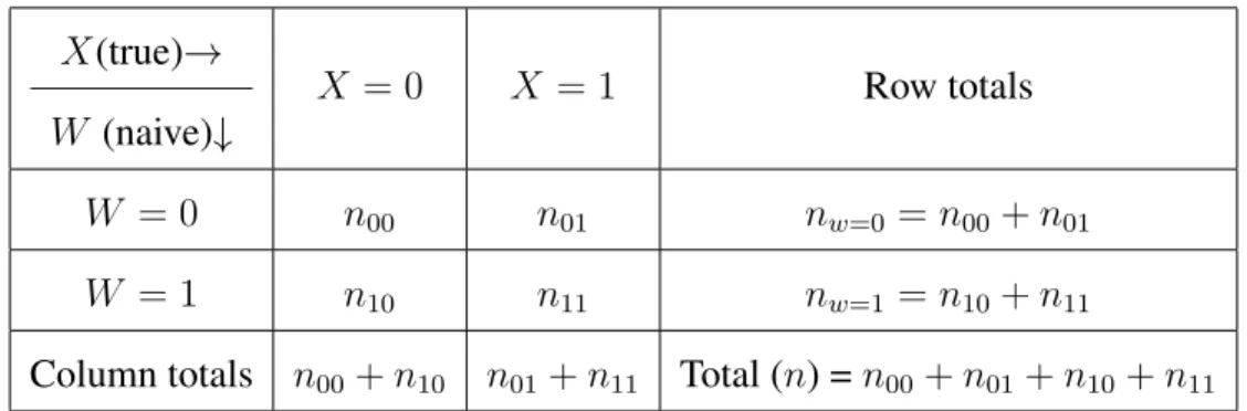
2X2 contingency tables from the validation data. The 2 X2 contingency table is constructed as follows:
Table 3.1:2X2 contingency table of binary variable subject to misclassificaiton
X(true)→ W (naive)↓
X = 0 X = 1 Row totals
W = 0 n00 n01 nw=0 =n00+n01 W = 1 n10 n11 nw=1 =n10+n11
Column totals n00+n10 n01+n11 Total (n) =n00+n01+n10+n11
wheren00denotes the number of observations whereW = 0andX = 0,n01denotes the number
of observations whereW = 0andX = 1,n10 denotes the number of observations whereW = 1
andX = 0andn11denotes the number of observations whereW = 1andX = 1. The conditional
probabilities of correct classification and misclassification are then calculated as follows:
ˆ π00 = n00 n00+n10 ˆ π10= 1−πˆ00 ˆ π11 = n11 n01+n11 ˆ π10= 1−π11ˆ (3.46)
Details of analysis of real data from the North Central Cancer Treatment Group (NCCTG) lung cancer clinical trial are provided in chapter 5.
Chapter 4
SIMULATION STUDY
A simulation study is conducted to evaluate the performance of the MC-SIMEX method in an AFT model where the survival time follows log-logistic distribution. In Section 4.1, we pro-pose a new method to simulate right censored survival data that is computationally less burdensome than existing methods and also saves processing time. Section 4.2 describes the methods used to estimate parameters. Section 4.3 describes the results of the performance of the original and modi-fied MC-SIMEX methods, followed by an analysis of robustness to misspecification of distribution in section 4.4. Section 4.5 describes the conclusion of our simulation study.
4.1 An overview of simulation methods
An overview of the existing simulation method and modified simulation method is pro-vided in sections 4.1.1 and 4.1.2 respectively.
4.1.1 Overview of the existing simulation method:
The existing simulation method generates survival times from a specific distribution and censoring times from a specific distribution (for e.g.: uniform) with an initial upper limit. The up-per limit is adjusted iteratively until the censoring up-percentage falls within the stipulated censoring range. To be more specific, if the censoring rate from a particular iteration is lesser than the lower bound of the stipulated range, then the upper limit is decreased so that the censoring rate increases and falls within the range. In the other case where the censoring rate is higher than the upper bound of the stipulated range, the upper limit is increased so that the censoring rate decreases and falls within the stipulated range. This process is repeated until an appropriate upper limit is reached.
We propose a new method to simulate right censored survival data, that achieves the exact level of censoring when the survival times follow a log-logistic distribution (however, this method can also be used for other survival data distributions). Existing algorithms require many number of iterations to achieve the desired censoring rates. The proposed algorithm, on the other hand, requires only one iteration to achieve the exact rate of censoring. Our algorithm also eases computational burden and saves processing time, as opposed to other algorithms. The proposed algorithm follows:
Step 1: Assign a value each forβ0,β1 andβ2.
Step 2: Generate n random values for the variableXwhich followsBernoullidistribution with the probability 0.5.
Step 3: Generate n random values for the variableZ which follows aN(0,1)distribution.
Step 4: Generate n random values for the variable(residual) which follows a logistic distribution with location zero and scale 1.
Step 5: Generate n natural logarithms of survival times using the following formula:
Y =β0 +β1X+β2Z+; whereY = logT.
Step 6: Generate n censoring times which follows aU ∼(0,10)distribution.
Step 7: Generate a new variable r = Y −log(c) for each of the n observations, where cis the censoring time.
Step 8: Pick the value of r that represents a percentile corresponding to the event rate. For exam-ple, if a censoring rate of 30% is desired, we will pick a value of r that corresponds to the 70th
percentile of its distribution.
Step 9: Create a new variable that represents the log of the new survival time which is obtained by deducting the value of r that represents the70thpercentile of its distribution from the original log of the survival time. Say,
logTnew =Y −rq70,
wherelogTnew represents the log of the new survival time, rq70 is the 70th percentile of the
dis-tribution of r. This step allows us to order the new survival times in such a way that 30% of the observations are censored and the remaining uncensored.
Step 10: Obtain a new survival time tnew by taking the exponential of the value of logT new
obtained from the previous step.
tnew = exp(logTnew).
Step 11: Generate a new variableynewwhich is the minimum oftnewand c, wherecis the censoring
time corresponding totnew.
Ynew =pmin(tnew, c).
Step 12: Fit an AFT model usingsurvreg[56] procedure in R (install MASS package[57] for sur-vival analysis before implementingsurvreg), withynewas the observed time, andδas the indicator
for censoring. If tnew > c then δ = 0, or else, δ takes on the value of 1. X and Z are the
ex-planatory variables. By the end of this step, the βˆnmisc (nmisc stands for no misclassification)
associated with the true variableX is obtained.
Step 13: Using themisclass[58] function in R, generate a naive variableW using the misclassifi-cation matrixΠ. Fit an AFT model as in Step 12, but with the naive covariateW instead ofX. By the end of this step,βˆnaive associated with the naive covariateW is obtained.
Step 14: Using themisclass function in R, generate additional naive covariatesW1, W2, W3 and W4from true covariateX. These naive covariates represent the misclassified form of the covariate Xatλ=0.8, 1.2, 1.6 and 2 respectively, whereλis the power of the misclassification matrixΠλ.
Step 15: At each level of misclassification, an AFT model is fit, as described in step 12, using the naive covariate instead of the true covariate. That is, four different AFT models using the naive covariatesW1,W2,W3andW4- one in each model, along with the confounding variableZare fit.
Step 16: Using the quadratic extrapolation function described in chapter 3, theβˆestimates (βˆW1,βˆW2,βˆW3
andβˆW4) obtained at the corresponding level of misclassification are extrapolated to a point on the
Y-axis whereλ= -1. The value ofβˆat this point on the Y-axis, is theβˆsimex estimate.
Step 17: 50 iterations[22] of steps 14 to 16 are run for each simulation. At the end of 50 iterations, average of theβˆsimex estimates is calculated to give the finalβˆsimexestimate for that simulation. In
addition, the empirical variance, estimated variance and Stefanski variance (VST) are also obtained
using equations 3.40-3.42, as described in chapter 3.
Step 18: At the end of one simulation and 50 replications within the simulation, the MSE, bias, estimated variance and coverage of the true estimator (βˆnmisc), the naive estimatorβˆnaive and the
ˆ
βsimex estimator are calculated.
Step 20: Steps 1 through 18 are repeated until a total of 500 Monte-Carlo runs are completed. The ˆ
βnmiscs, βˆWs andβˆsimexs along with their corresponding MSEs, biases, estimated variances ,
em-pirical variances and coverages are averaged over 500 Monte-Carlo runs to give the corresponding final estimates.
the start of section 4.1.2), it must be noted that this algorithm also results in a distortion of the value of the intercept in the model. However, since the study of properties of the intercept is not our primary objective, we ignore this distortion. The properties of β1 and β2 remain unchanged
despite this adjustment. The distribution of the newly generated survival times also remains the same, albeit a change in the expected value (mean) occurs.
4.2 Data simulation and estimation of parameters
In this study, a sample size of 200 is chosen. We consider two covariates, one binary and the other continuous. The binary covariate X, which is subject to misclassification error, is generated from a binomial distribution (X ∼ binom(n,0.5)). The continuous covariate Z is generated from a standard normal distribution(Z ∼ N(0,1)), independent of X. The error term
i is generated from a standard logistic distribution with i ∼ logistic(0,1) (0 is the value of
the location parameter and 1 is the value of the scale parameter). The survival timesT are then generated using the following equation:
Y =log(T) =β0+β1X+β2Z +i
T = exp(Y),
where the values of β1 andβ2 are pre-specified. The censoring timescare generated from a
uni-form distribution withc∼U(0,10).
After conducting this preliminary simulation, the algorithm described in steps 7 through 13 of section 4.1.2 is performed. That is, a new variabler=Y −log(c)is created followed by the selection of the value ofr, which corresponds to a stipulated percentile of its distribution, sayrq70.
This is followed by the creation of a new variablelogTnew, that represents the difference between
the variableY andrq70. The new survival time,tnew is then obtained by taking the exponential of
the variable logTnew. Censoring statuses are then assigned and an AFT model is fit, as described
In this dissertation, two situations are considered, wherein the misclassification matri-ces are 0.8 0.2 0.2 0.8 and 0.9 0.3 0.1 0.7
. Estimates ofβ1 are obtained for each Monte Carlo run using the true estimator (which is obtained from the AFT model using the true covariateX), naive esti-mator (which is obtained from the AFT model using the naive covariateW) and the MC- SIMEX estimator. Also, for each run, the corresponding bias and MSE are obtained. In order to obtain the MC-SIMEX estimator, a total of 50 replications were run for each simulation, as done by Slate et al[22]. A total of 500 simulations were run. The estimates of βˆnmisc, βˆnaive andβˆsimex and their
corresponding bias and MSE are obtained as follows:
ˆ βnmisc= 1 M M X i=1 ˆ βnmisci ˆ βnaive = 1 M M X i=1 ˆ βnaivei ˆ βsimex = 1 M M X i=1 ˆ βsimexi ˆ M SEnmisc= 1 M M X i=1 ( ˆβnmisci−(β)) 2 ˆ M SEnaive = 1 M M X i=1 ( ˆβnaivei −(β)) 2 ˆ M SEsimex = 1 M M X i=1 ( ˆβsimexi−(β)) 2 ˆ biasnmisc= 1 M M X i=1 ( ˆβnmisci −β) ˆ biasnaive = 1 M M X i=1 ( ˆβnaivei−β) ˆ biassimex = 1 M M X i=1 ( ˆβsimexi −β)
The coverage probability of each estimator is then obtained by first estimating the variance and standard error (SE) of each estimator from the information matrix, as described in section 3.3 of chapter 3. 95% confidence intervals are then estimated by using the following formula:
95%CI = ˆβ±1.96SE
The coverage probability is then calculated as the percentage of the occurrences where the 95% CI includes the value of the true parameter.
4.3 Results of the performance of the original and modified MC-SIMEX
estimator
Tables 4.1 - 4.4 illustrate the results of the MC-SIMEX procedure when the survival times follow standard log-logistic distribution for 0%, 30%, 50% and 70% levels of censoring, with the true Π being
0.8 0.2 0.2 0.8
. Table 4.5 and table 4.6 illustrate the results of the modified MC-SIMEX procedure, under similar specifications as table 4.1 and 4.2. Tables 4.7 - 4.10 illus-trate the results of the MC-SIMEX procedure when the survival times follow standard log-logistic distribution for 0%, 30%, 50% and 70% levels of censoring, with the true Π being
0.9 0.3 0.1 0.7 . Table 4.11 and table 4.12 illustrate the results of the modified MC-SIMEX procedure, under simi-lar specifications as table 4.7 and table 4.8.
4.3.1 Results for a sensitivity of 80% and specificity of 80%:
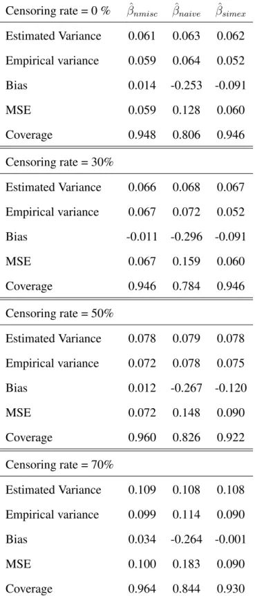
The performance of the MC-SIMEX estimator is evaluated for four different combi-nations of β1 and β2, those being: β1 = −log 2 and β2 = 0.5, β1 = −log 2 and β2 = −0.5,
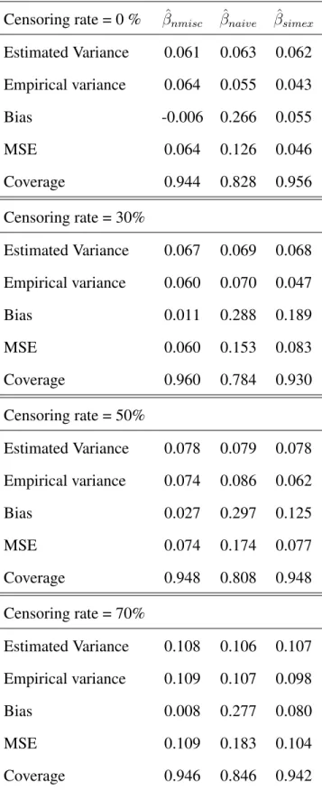
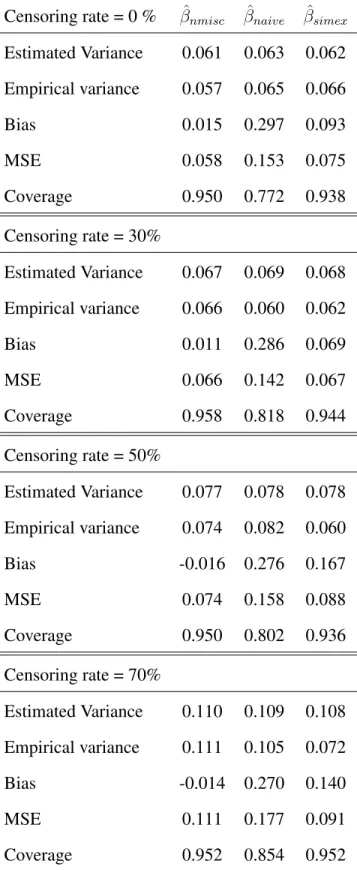
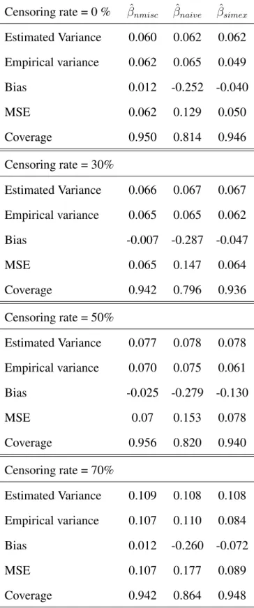
β1 = log 2and β2 = 0.5and finally,β1 = log 2and β2 = −0.5. For aΠ of 0.8 0.2 0.2 0.8 , tables 4.1 - 4.4 show that the MC-SIMEX estimator consistently performs better than the naive estimator. The magnitude of the bias associated with the MC-SIMEX estimator is always lower than that of the naive estimator. The MSE associated with the MC-SIMEX estimator is consistently lower than that of the naive estimator across all levels of censoring. With regard to the coverage probabilities, the MC-SIMEX estimator is shown to perform satisfactorily and consistently better than the naive estimator across all levels of censoring.
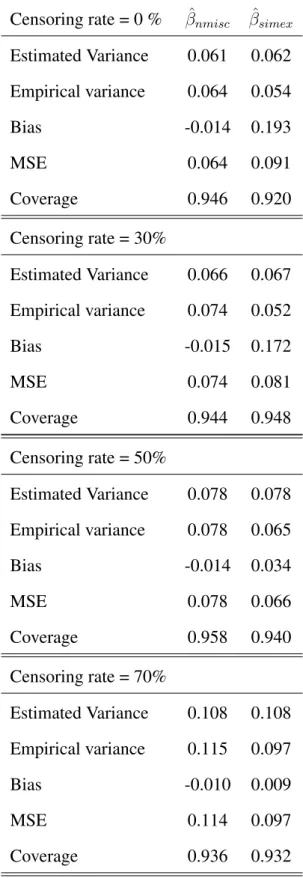
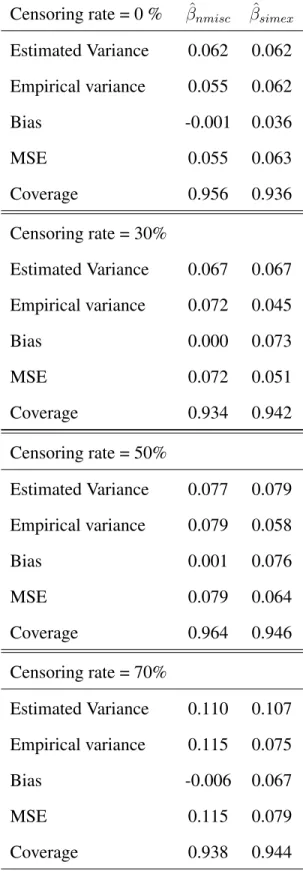
Table 4.5 and table 4.6 illustrate the performance of the modified SIMEX procedure using the log-logistic distribution of survival times for a specified true sensitivity of 80%and a true specificity of 80%. It can be seen from table 4.5 and table 4.6 that the bias, MSE and coverage probabilities for the modified SIMEX procedure are satisfactory and comparable to that of the true estimator. A comparison of tables 4.5 and 4.6 to tables 4.1 and 4.2 shows that the performance of the modified MC-SIMEX procedure is comparable to the performance of the original MC-SIMEX procedure and that there are no notable deviations in bias, MSE and coverage probabilities.
Table 4.1: Results of the MC-SIMEX procedure using log-logistic distribution of survival times. Sensitivity =80%, Specificity =80%. Trueβ values areβ1 =−log 2, β2 = 0.5
Censoring rate = 0 % βˆnmisc βˆnaive βˆsimex
Estimated Variance 0.061 0.063 0.062 Empirical variance 0.064 0.055 0.043 Bias -0.006 0.266 0.055 MSE 0.064 0.126 0.046 Coverage 0.944 0.828 0.956 Censoring rate = 30% Estimated Variance 0.067 0.069 0.068 Empirical variance 0.060 0.070 0.047 Bias 0.011 0.288 0.189 MSE 0.060 0.153 0.083 Coverage 0.960 0.784 0.930 Censoring rate = 50% Estimated Variance 0.078 0.079 0.078 Empirical variance 0.074 0.086 0.062 Bias 0.027 0.297 0.125 MSE 0.074 0.174 0.077 Coverage 0.948 0.808 0.948 Censoring rate = 70% Estimated Variance 0.108 0.106 0.107 Empirical variance 0.109 0.107 0.098 Bias 0.008 0.277 0.080 MSE 0.109 0.183 0.104 Coverage 0.946 0.846 0.942
Table 4.2: Results of the MC-SIMEX procedure using log-logistic distribution of survival times. Sensitivity =80%, Specificity =80%. Trueβ values areβ1 =−log 2, β2 =−0.5
Censoring rate = 0 % βˆnmisc βˆnaive βˆsimex
Estimated Variance 0.061 0.063 0.062 Empirical variance 0.057 0.065 0.066 Bias 0.015 0.297 0.093 MSE 0.058 0.153 0.075 Coverage 0.950 0.772 0.938 Censoring rate = 30% Estimated Variance 0.067 0.069 0.068 Empirical variance 0.066 0.060 0.062 Bias 0.011 0.286 0.069 MSE 0.066 0.142 0.067 Coverage 0.958 0.818 0.944 Censoring rate = 50% Estimated Variance 0.077 0.078 0.078 Empirical variance 0.074 0.082 0.060 Bias -0.016 0.276 0.167 MSE 0.074 0.158 0.088 Coverage 0.950 0.802 0.936 Censoring rate = 70% Estimated Variance 0.110 0.109 0.108 Empirical variance 0.111 0.105 0.072 Bias -0.014 0.270 0.140 MSE 0.111 0.177 0.091 Coverage 0.952 0.854 0.952
Table 4.3: Results of the MC-SIMEX procedure using log-logistic distribution of survival times. Sensitivity =80%, Specificity =80%. Trueβ values areβ1 = log 2, β2 = 0.5
Censoring rate = 0 % βˆnmisc βˆnaive βˆsimex
Estimated Variance 0.060 0.062 0.062 Empirical variance 0.062 0.065 0.049 Bias 0.012 -0.252 -0.040 MSE 0.062 0.129 0.050 Coverage 0.950 0.814 0.946 Censoring rate = 30% Estimated Variance 0.066 0.067 0.067 Empirical variance 0.065 0.065 0.062 Bias -0.007 -0.287 -0.047 MSE 0.065 0.147 0.064 Coverage 0.942 0.796 0.936 Censoring rate = 50% Estimated Variance 0.077 0.078 0.078 Empirical variance 0.070 0.075 0.061 Bias -0.025 -0.279 -0.130 MSE 0.07 0.153 0.078 Coverage 0.956 0.820 0.940 Censoring rate = 70% Estimated Variance 0.109 0.108 0.108 Empirical variance 0.107 0.110 0.084 Bias 0.012 -0.260 -0.072 MSE 0.107 0.177 0.089 Coverage 0.942 0.864 0.948
Table 4.4: Results of the MC-SIMEX procedure using log-logistic distribution of survival times. Sensitivity =80%, Specificity =80%. Trueβ values areβ1 = log 2, β2 =−0.5
Censoring rate = 0 % βˆnmisc βˆnaive βˆsimex
Estimated Variance 0.061 0.063 0.062 Empirical variance 0.059 0.064 0.052 Bias 0.014 -0.253 -0.091 MSE 0.059 0.128 0.060 Coverage 0.948 0.806 0.946 Censoring rate = 30% Estimated Variance 0.066 0.068 0.067 Empirical variance 0.067 0.072 0.052 Bias -0.011 -0.296 -0.091 MSE 0.067 0.159 0.060 Coverage 0.946 0.784 0.946 Censoring rate = 50% Estimated Variance 0.078 0.079 0.078 Empirical variance 0.072 0.078 0.075 Bias 0.012 -0.267 -0.120 MSE 0.072 0.148 0.090 Coverage 0.960 0.826 0.922 Censoring rate = 70% Estimated Variance 0.109 0.108 0.108 Empirical variance 0.099 0.114 0.090 Bias 0.034 -0.264 -0.001 MSE 0.100 0.183 0.090 Coverage 0.964 0.844 0.930
Table 4.5: Results of the modified MC-SIMEX procedure using log-logistic distribution of survival times. Sensitivity =80%, Specificity =80%. Trueβ values areβ1 =−log 2, β2 = 0.5
Censoring rate = 0 % βˆnmisc βˆsimex
Estimated Variance 0.061 0.062 Empirical variance 0.064 0.054 Bias -0.014 0.193 MSE 0.064 0.091 Coverage 0.946 0.920 Censoring rate = 30% Estimated Variance 0.066 0.067 Empirical variance 0.074 0.052 Bias -0.015 0.172 MSE 0.074 0.081 Coverage 0.944 0.948 Censoring rate = 50% Estimated Variance 0.078 0.078 Empirical variance 0.078 0.065 Bias -0.014 0.034 MSE 0.078 0.066 Coverage 0.958 0.940 Censoring rate = 70% Estimated Variance 0.108 0.108 Empirical variance 0.115 0.097 Bias -0.010 0.009 MSE 0.114 0.097 Coverage 0.936 0.932
Table 4.6: Results of the modified MC-SIMEX procedure using log-logistic distribution of survival times. Sensitivity =80%, Specificity =80%. Trueβ values areβ1 =−log 2, β2 =−0.5
Censoring rate = 0 % βˆnmisc βˆsimex
Estimated Variance 0.062 0.062 Empirical variance 0.055 0.062 Bias -0.001 0.036 MSE 0.055 0.063 Coverage 0.956 0.936 Censoring rate = 30% Estimated Variance 0.067 0.067 Empirical variance 0.072 0.045 Bias 0.000 0.073 MSE 0.072 0.051 Coverage 0.934 0.942 Censoring rate = 50% Estimated Variance 0.077 0.079 Empirical variance 0.079 0.058 Bias 0.001 0.076 MSE 0.079 0.064 Coverage 0.964 0.946 Censoring rate = 70% Estimated Variance 0.110 0.107 Empirical variance 0.115 0.075 Bias -0.006 0.067 MSE 0.115 0.079 Coverage 0.938 0.944
4.3.2 Results for a sensitivity of 90% and specificity of 70%:
Tables 4.7-4.10 illustrate the performance of the MC-SIMEX estimator in comparison to the naive estimator, whenΠis
0.9 0.3 0.1 0.7
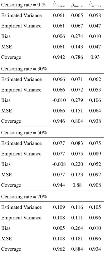
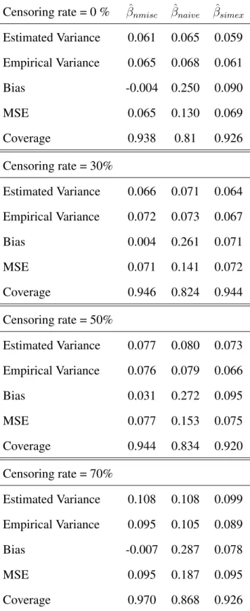
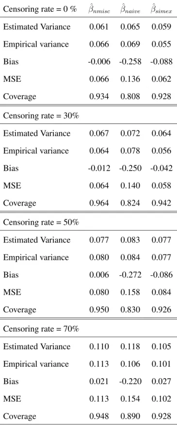
. The magnitude of the bias associated with the MC-SIMEX estimator is consistently lower than that of the naive estimator at all the levels of censoring. The MSE associated with the MC-SIMEX etimator is also consistently lower than that of the naive estimator. The coverage probability associated with the MC-SIMEX estimator is satisfactory and consistently better than that of the naive estimator at all levels of censoring.
Table 4.11 and table 4.12 illustrate the performance of the modified SIMEX procedure using the log-logistic distribution of survival times for a specified true sensitivity of 90% and a true specificity of 70%. It can be seen from table 4.11 and table 4.12 that bias, MSE and coverage probabilities associated with the modified MC-SIMEX procedure are satisfactory and comparable to that of the true estimator. A comparison of tables 4.11 and 4.12 to tables 4.7 and 4.8 shows that the performance of the modified MC-SIMEX procedure is comparable to that of the original MC-SIMEX procedure and that there are no notable deviations.
4.4 Robustness
In this dissertation, the analysis of robustness is done in by mis-specifying a log-logistic distribution (of survival time), as a Weibull distribution. The results of this misspecification of survival time distribution are described in this section.
Table 4.7: Results of the MC-SIMEX procedure using log-logistic distribution of survival times. Sensitivity =90%, Specificity =70%. Trueβ values areβ1 =−log 2, β2 = 0.5
Censoring rate = 0 % βˆnmisc βˆnaive βˆsimex
Estimated Variance 0.061 0.065 0.058 Empirical Variance 0.061 0.067 0.047 Bias 0.006 0.274 0.010 MSE 0.061 0.143 0.047 Coverage 0.942 0.786 0.93 Censoring rate = 30% Estimated Variance 0.066 0.071 0.062 Empirical Variance 0.066 0.072 0.053 Bias -0.010 0.279 0.106 MSE 0.066 0.151 0.064 Coverage 0.946 0.804 0.938 Censoring rate = 50% Estimated Variance 0.077 0.083 0.075 Empirical Variance 0.077 0.075 0.089 Bias -0.008 0.220 0.052 MSE 0.077 0.123 0.092 Coverage 0.944 0.88 0.908 Censoring rate = 70% Estimated Variance 0.109 0.116 0.105 Empirical Variance 0.108 0.111 0.096 Bias 0.005 0.264 0.010 MSE 0.108 0.181 0.096 Coverage 0.962 0.884 0.934
Table 4.8: Results of the MC-SIMEX procedure using log-logistic distribution of survival times. Sensitivity =90%, Specificity =70%. Trueβ values areβ1 =−log 2, β2 =−0.5
Censoring rate = 0 % βˆnmisc βˆnaive βˆsimex
Estimated Variance 0.061 0.065 0.059 Empirical Variance 0.065 0.068 0.061 Bias -0.004 0.250 0.090 MSE 0.065 0.130 0.069 Coverage 0.938 0.81 0.926 Censoring rate = 30% Estimated Variance 0.066 0.071 0.064 Empirical Variance 0.072 0.073 0.067 Bias 0.004 0.261 0.071 MSE 0.071 0.141 0.072 Coverage 0.946 0.824 0.944 Censoring rate = 50% Estimated Variance 0.077 0.080 0.073 Empirical Variance 0.076 0.079 0.066 Bias 0.031 0.272 0.095 MSE 0.077 0.153 0.075 Coverage 0.944 0.834 0.920 Censoring rate = 70% Estimated Variance 0.108 0.108 0.099 Empirical Variance 0.095 0.105 0.089 Bias -0.007 0.287 0.078 MSE 0.095 0.187 0.095 Coverage 0.970 0.868 0.926
Table 4.9: Results of the MC-SIMEX procedure using log-logistic distribution of survival times. Sensitivity =90%, Specificity =70%. Trueβ values areβ1 = log 2, β2 = 0.5
Censoring rate = 0 % βˆnmisc βˆnaive βˆsimex
Estimated Variance 0.061 0.065 0.059 Empirical variance 0.066 0.069 0.055 Bias -0.006 -0.258 -0.088 MSE 0.066 0.136 0.062 Coverage 0.934 0.808 0.928 Censoring rate = 30% Estimated Variance 0.067 0.072 0.064 Empirical variance 0.064 0.078 0.056 Bias -0.012 -0.250 -0.042 MSE 0.064 0.140 0.058 Coverage 0.964 0.824 0.942 Censoring rate = 50% Estimated Variance 0.077 0.083 0.077 Empirical variance 0.080 0.084 0.077 Bias 0.006 -0.272 -0.086 MSE 0.080 0.158 0.084 Coverage 0.950 0.830 0.926 Censoring rate = 70% Estimated Variance 0.110 0.118 0.105 Empirical variance 0.113 0.106 0.101 Bias 0.021 -0.220 0.027 MSE 0.113 0.154 0.102 Coverage 0.948 0.890 0.928
Table 4.10: Results of the MC-SIMEX procedure using log-logistic distribution of survival times. Sensitivity =90%, Specificity =70%. Trueβ values areβ1 = log 2, β2 =−0.5
Censoring rate = 0 % βˆnmisc βˆnaive βˆsimex
Estimated Variance 0.061 0.065 0.059 Empirical variance 0.061 0.066 0.053 Bias -0.003 -0.262 -0.085 MSE 0.061 0.134 0.060 Coverage 0.932 0.810 0.912 Censoring rate = 30% Estimated Variance 0.066 0.071 0.063 Empirical variance 0.061 0.074 0.070 Bias 0.016 -0.243 -0.187 MSE 0.061 0.133 0.104 Coverage 0.950 0.830 0.904 Censoring rate = 50% Estimated Variance 0.078 0.084 0.075 Empirical variance 0.082 0.085 0.080 Bias 0.010 -0.247 -0.070 MSE 0.082 0.146 0.085 Coverage 0.944 0.854 0.920 Censoring rate = 70% Estimated Variance 0.110 0.117 0.110 Empirical variance 0.091 0.104 0.114 Bias 0.018 -0.243 -0.012 MSE 0.091 0.163 0.114 Coverage 0.964 0.896 0.926
Table 4.11:Results of the modified MC-SIMEX procedure using log-logistic distribution of survival times. Sensitivity =90%, Specificity =70%. Trueβ values areβ1 =−log 2, β2 = 0.5
Censoring rate = 0 % βˆnmisc βˆsimex
Estimated Variance 0.060 0.057 Empirical variance 0.070 0.065 Bias -0.018 0.123 MSE 0.070 0.080 Coverage 0.936 0.904 Censoring rate = 30% Estimated Variance 0.066 0.061 Empirical variance 0.068 0.074 Bias -0.003 0.086 MSE 0.067 0.081 Coverage 0.946 0.916 Censoring rate = 50% Estimated Variance 0.077 0.072 Empirical variance 0.078 0.069 Bias -0.015 0.044 MSE 0.078 0.071 Coverage 0.946 0.938 Censoring rate = 70% Estimated Variance 0.107 0.097 Empirical variance 0.111 0.107 Bias 0.023 0.067 MSE 0.111 0.112 Coverage 0.956 0.942
Table 4.12:Results of the modified MC-SIMEX procedure using log-logistic distribution of survival times. Sensitivity =90%, Specificity =70%. Trueβ values areβ1 =−log 2, β2 =−0.5
Censoring rate = 0 % βˆnmisc βˆsimex
Estimated Variance 0.061 0.059 Empirical variance 0.062 0.059 Bias 0.001 0.106 MSE 0.062 0.070 Coverage 0.944 0.906 Censoring rate = 30% Estimated Variance 0.065 0.063 Empirical variance 0.072 0.066 Bias 0.001 0.070 MSE 0.072 0.070 Coverage 0.924 0.922 Censoring rate = 50% Estimated Variance 0.078 0.072 Empirical variance 0.083 0.085 Bias -0.017 0.065 MSE 0.083 0.089 Coverage 0.942 0.926 Censoring rate = 70% Estimated Variance 0.109 0.098 Empirical variance 0.114 0.070 Bias -0.007 0.041 MSE 0.114 0.071 Coverage 0.952 0.948
Tables 4.13 to 4.16 illustrate the effect of misspecification of a log-logistic distribution as a Weibull distribution, for 0%, 30%, 50% and 70% levels of censoring. In tables 4.13 and 4.14, the misclassification matrix used is
0.8 0.2 0.2 0.8
, while in tables 4.15 and 4.16, the
misclas-sification matrix used is 0.9 0.3 0.1 0.7
. This analysis of robustness is done for two combinations of pre-specifiedβ1 andβ2 values. Tables 4.13 to 4.16 show that the MC-SIMEX procedure performs
consistently better than the naive estimator in terms of bias, MSE and coverage probabilities and also that the MC-SIMEX procedure is robust to mis-specification of distribution and change in parameter values.
4.5 Conclusion
Tables 4.1 to 4.16 show that the MC-SIMEX estimator is a reliable and valid estimator even under misspecification of distribution. The above tables also show that under varying degrees of misclassification of the binary variableX and at varying levels of censoring, the MC-SIMEX estimates are very close to the true value ofβs that are assigned in the simulation. Theβˆestimates obtained from our modified MC-SIMEX method also proved to be efficient and comparable to the true estimator. However, we will be remiss, if we didn’t note the increased bias in the MC-SIMEX estimates, when dealing with a mis-specified distribution. We attribute this finding to chance and reiterate that such findings are not totally surprising, given that similar findings have been reported in the study by Slate et. al.[22]
Table 4.13:Results of the MC-SIMEX procedure with the log-logistic distribution of survival times, but misspecified as a Weibull distribution. Sensitivity =80%, Specificity =80%. Trueβ values are β1 =−log 2, β2 = 0.5
Censoring rate = 0 % βˆnmisc βˆnaive βˆsimex
Estimated Variance 0.061 0.063 0.114 Empirical variance 0.065 0.067 0.122 Bias 0.006 0.277 0.124 MSE 0.065 0.143 0.137 Coverage 0.942 0.796 0.922 Censoring rate = 30% Estimated Variance 0.066 0.068 0.064 Empirical variance 0.065 0.068 0.070 Bias -0.003 0.281 0.070 MSE 0.065 0.148 0.075 Coverage 0.948 0.802 0.922 Censoring rate = 50% Estimated Variance 0.078 0.079 0.070 Empirical variance 0.074 0.087 0.062 Bias 0.003 0.292 0.171 MSE 0.074 0.172 0.091 Coverage 0.958 0.802 0.916 Censoring rate = 70% Estimated Variance 0.110 0.108 0.097 Empirical variance 0.115 0.112 0.068 Bias 0.006 0.286 0.189 MSE 0.115 0.193 0.104 Coverage 0.948 0.834 0.934
Table 4.14: Results of the MC-SIMEX procedure with the log-logistic distribution distribution of survival times, but misspecified as a Weibull distribution. Sensitivity = 80%, Specificity = 80%. Trueβ valuesβ1 =−log 2, β2 =−0.5
Censoring rate = 0 % βˆnmisc βˆnaive βˆsimex
Estimated Variance 0.061 0.062 0.111 Empirical variance 0.059 0.064 0.101 Bias -0.003 0.268 0.114 MSE 0.059 0.135 0.113 Coverage 0.954 0.818 0.924 Censoring rate = 30% Estimated Variance 0.066 0.067 0.064 Empirical variance 0.063 0.068 0.055 Bias 0.015 0.294 0.130 MSE 0.063 0.154 0.071 Coverage 0.954 0.782 0.944 Censoring rate = 50% Estimated Variance 0.078 0.079 0.070 Empirical variance 0.074 0.087 0.062 Bias 0.003 0.292 0.171 MSE 0.074 0.172 0.091 Coverage 0.958 0.802 0.916 Censoring rate = 70% Estimated Variance 0.108 0.106 0.098 Empirical variance 0.099 0.096 0.062 Bias 0.018 0.313 0.089 MSE 0.099 0.193 0.070 Coverage 0.956 0.846 0.950