Peer Effects in Math and Science
∗
∗
∗
∗
Juanna Schrøter Joensen
Stockholm School of Economics
Helena Skyt Nielsen
Aarhus University
April 21, 2015
Abstract:
This paper examines how skills are shaped by social interactions in schools and families. We focus on critical course choices in high school and naturally occurring peer groups. We overcome the identification challenges of estimating peer effects in education by exploiting exogenous variation in choice sets. First, we analyze a universal free-choice reform causing a fall in math-science skills. We show how it amplified the falling skill supply in peer groups with a stronger math-science norm, particularly for boys. Second, the detailed nature of our administrative data allows us to analyze the underlying mechanisms. We exploit quasi-experimental variation stemming from a pre-reform pilot scheme. The pilot induced a random subset of older siblings to choose advanced math-science at a lower cost, while not directly affecting the course choices of younger siblings. Therefore, any influences of the pilot on the younger siblings may be attributed to the peer influence of the older sibling. We find that younger siblings are 2-3 percentage points more likely to choose math-science if their older sibling unexpectedly could choose math-science at a lower cost. Spillovers are strongest among closely spaced siblings, in particular brothers. We argue that competition is likely the driving force behind younger siblings conforming to their older siblings’ choices.
JEL Classification: I21, I24, J24, J16, J12, Z13.
Keywords: Social interaction, extrinsic and intrinsic incentives, siblings, high school curriculum, skill formation.
∗
Contact details: Joensen, Department of Economics, Stockholm School of Economics, email: [email protected]. Nielsen: Department of Economics and Business, Aarhus University, email: [email protected]. We appreciate enlightening discussions with and comments from Anders Björklund, Tore Ellingsen, Ina Ganguli, Leonie Gerhards, Maria Knoth Humlum, Eric Maurin, Magne Mogstad, Julia Nafziger, Torsten Persson, Barbara Petrongolo, and participants at SOLE 2014, ELE 2014, IWAEE 2013 and seminar participants at the CEP-LSE Education Group, Copenhagen Business School, Federal Reserve Bank of New York, IIES Stockholm University, Lancaster University, Oslo University, Stavanger University, SOFI Stockholm University, Sussex University, University of Southern Denmark, York University, and Aarhus University.We thank Kasper Jørgensen and Pernille Hansen for research assistance. The usual disclaimers apply.
1
1.
Introduction
Social interactions may play an important role in the formation of skills. Peer groups may either transmit information about particular educational investments or carry social norms and identity concerns influencing an individual’s educational decision. Social interactions may reinforce or counteract the direct effect of economic shocks or policy interventions. As a consequence, social interaction effects may have contributed to the increased inequality and the sluggish skill development in terms of slowing down both college preparedness and college enrollment (Goldin and Katz, 2008).
In this paper, we focus on social interactions within the family and schools. The context is advanced math-science choices in high school.1 We overcome the identification challenges of estimating peer effects in education by exploiting plausibly exogenous variation in choice sets stemming from a universal and uniform free-choice reform and a pre-reform pilot program offering one extra course combination. Our contribution is twofold: First, we specify and test a model of how skill supply is shaped by institutions and their interactions with the social environment in which individuals make their educational choices. We show how the free-choice reform caused a fall in math-science skills which was amplified in peer groups with a stronger math-science norm, particularly for boys. Second, we investigate the underlying mechanisms by estimating causal sibling spillover effects. We show that the pilot offered a random subset of older siblings the choice of advanced math-science at a lower cost, while not directly affecting the course choices of younger siblings. We find that between one third and half of the direct effect on the older sibling spills over on the younger siblings through social interactions. Spillovers are strongest among closely spaced siblings, in particular brothers.
We set up a model of how individual educational choices are determined by not only extrinsic incentives (material costs and benefits), but also intrinsic incentives (identity and social norms) and their interaction. Extrinsic incentives depend on the monetary payoff as well as curricula which not only impact costs and benefits of educational choices directly, but also send signals about the values of schools and society. Intrinsic incentives depend on individuals’ social environment; primarily,
1
This choice is a prerequisite for increasing the supply of college graduates in science, technology, engineering, and mathematics (STEM). Any policy aiming to increase the investment in math and science skills (e.g. increased course requirements implemented in the US following A Nation at Risk, Gardner et al., 1983) may be seriously dampened or amplified by social interaction effects. Social interaction effects are extremely important during the teenage years when decisions on more advanced coursework are taken (Card and Giuliano, 2013; Akerlof, 1997; Akerlof and Kranton, 2002).
2
siblings and parents, but also schoolmates. Younger siblings get a utility gain (loss) of (not) conforming to their older sibling and the identity payoff depends on how many conformers are in their peer group. Our model builds on the theoretical framework of two recent papers by Benabou and Tirole (2011) and Jia and Persson (2014) where conformity arises endogenously in equilibrium as individuals infer the social norm from their peers’ educational choices.2 Empirical evidence of the relevance of these mechanisms is scarce, but pivotal for better understanding how economic shocks and policy interventions influence educational decisions.3 To the best of our knowledge, this is the first paper to quantify the importance of siblings and peers on educational choices with a considerable career impact.
We exploit a universal and uniform high school reform in Denmark in 1988 to investigate the empirical relevance of the model. We find evidence that extrinsic incentives are more strongly crowded in for younger brothers and sibling pairs where the older sibling chose advanced math and science. Furthermore, there appears to be more social pressure on boys to choose math and science in the baseline. A more restrictive model imposing uniform complementarity could not have explained these facts. We show how our model can explain these two facts and how the free choice has contributed to the gender convergence in math and science skills.
Having established how educational choice depends on and interacts with the social environment, we turn to understanding the underlying mechanisms by estimating causal sibling spillover effects. Estimating causal peer effects is challenging due to simultaneity, correlated unobservables, and endogenous peer group membership (Manski, 1993; 1995). We study naturally occurring peer groups and exploit exogenous variation in the cost of taking up advanced math and science in high school among a partial population (Moffitt, 2001).4
We exploit the fact that some older siblings in Denmark in 1984-87 were unexpectedly exposed to a pilot scheme after entering high school and investigate whether they influenced the course choices of their younger siblings. In previous work (Joensen and Nielsen, 2009; 2014) we employed this pilot scheme to investigate the impact on the individuals’ own educational choices, subsequent
2
This is different from the related paper by Akerlof and Kranton (2002) who introduce identity into a model of educational choice, but impose complementarity as individuals gain utility from fitting into a social group.
3
The discussion of peer effects in education dates back at least to the controversial Coleman report (Coleman et al., 1966). Recent reviews are provided by Moffitt (2001) and Sacerdote (2011). Most of the literature focuses on student test scores or risky behavior as outcomes. We focus on educational choices that have economically important impacts on future careers and employ a theoretically founded empirical strategy to identify peer effects in educational choice.
4
Our study is thus methodologically similar to the study of social interaction effects in program participation by Dahl, Løken and Mogstad (2014), Avvisati, Gurgand, Guyon and Maurin (2014), and Dahl, Kostøl and Mogstad (2014).
3
careers, and earnings. Those unexpectedly exposed to the pilot scheme obtained more advanced college degrees and substantially higher earnings. In this paper, we analyze whether there were spillover effects on younger siblings who were unexposed themselves. Any influence of this pilot scheme on younger siblings’ course choices can be interpreted as a causal peer effect, since the pilot scheme only directly reduced the cost of choosing advanced math and science for older siblings. The exogenous increase in extrinsic incentives for the older sibling is thus essentially an increase in intrinsic incentives for the younger sibling in the presence of identity concerns and a utility cost of not conforming. We find that younger siblings are 2-3 percentage points more likely to choose math and science if their older sibling was exposed to the pilot scheme. Since the first-stage estimate is around 7 percentage points, this implies a peer influence of older siblings on younger siblings of about 0.35-0.55. This means that by affecting the choice of the older sibling, about half of the effect is expected to spill over on the younger sibling’s choice. More generally, this suggests that knowledge about the social peer group is important to predict the total impact of education policies. Policies targeted at influential peers (such as older siblings) would have more widespread effects.
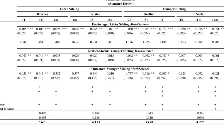
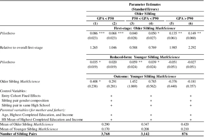
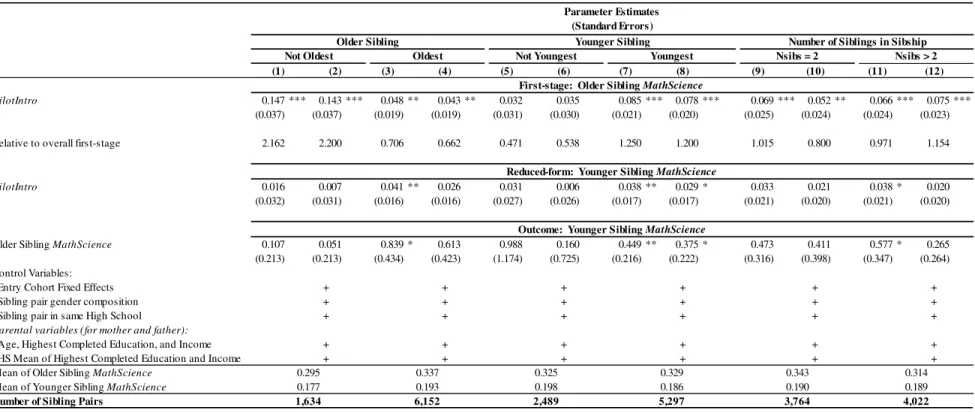
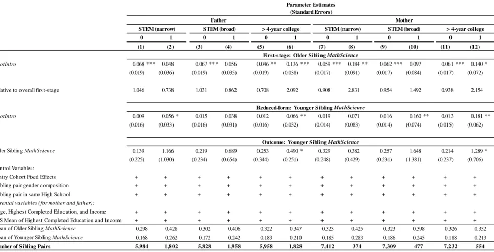
Our results suggest that there is substantial heterogeneity in peer effects – both in terms of how strongly the older sibling responds to extrinsic incentives and how their choice spills over on the younger sibling through intrinsic incentives. The causal peer effects persist among closely spaced siblings, and the significance depends on the gender composition of the sibling pair. Peer effects are largest for relatively closely spaced brothers. First-born siblings are the most influential peers and parental education is also important for spillovers. We provide suggestive evidence that sibling competition is likely driving the peer effect as younger siblings are less likely to conform to their older sibling’s course choice if the older sibling is among the top performers.
Our paper speaks to the literature trying to unravel the role of the family in skill formation and human development more generally.5 However, traditionally the child is not modelled as interacting
with siblings, and rigorous economics research on the importance of social interactions among siblings is scarce.6 We document that sibling spillovers are possibly large and we provide a
5 See e.g. Becker and Tomes (1979, 1986), Cunha and Heckman (2007), Cunha et al. (2010) for a theoretical framework.
Heckman and Mosso (2014) provide a recent review.
6
Butcher and Case (1994) find that the presence of a sister in the sibship reduces education of daughters, and they argue that this is because a sister changes the reference group. Qureshi (2013) finds that the education of older sisters improves the education of younger brothers, and she argues that this result reflects improved quality of child care as the older sister takes care of younger siblings. Sibling spillover effects have also been documented from parental leave taking among brothers (Dahl, Mogstad and Løken, 2014), from newborn health (Breining, Daysal, Simonsen and Trandafir, 2015) and adolescent smoking, drinking and marijuana use (Altonji, Cattan and Ware, 2013).
4
framework for understanding the plausible mechanisms. Our results have implications for understanding equality of opportunity, inequality, and intergenerational mobility where the importance of family background for educational investments has long been recognized and sibling correlations in schooling have recently been examined.7 We go beyond simple sibling correlations and estimate causal effects in order to understand the complex family component that siblings share.
The remainder of the paper unfolds as follows: Section 2 specifies and tests the predictions of an economic model of educational choices and peer effects. Section 3 discusses identification of social interaction effects and presents the institutional background which our empirical strategy relies on. Section 4 describes the data, while section 5 presents the empirical analysis of social interaction effects in the choice of math and science in high school. Section 6 investigates mechanisms and heterogeneity in peer effects. Section 7 concludes the paper.
2.
A Framework Linking Educational Choices and Peer Effects
In this section we lay out an economic model of how an individual makes educational choices conditional on the institutions and social environment. We derive two model predictions and provide empirical evidence for their relevance by use of exogenous variation from a high school reform implemented in 1988. We investigate course choice responses to this reform across different peer groups with presumably different social norms and different costs of not conforming.
Our model describes how an individual’s choice can be determined by extrinsic and intrinsic incentives and their interaction. Extrinsic incentives include monetary payoff and curriculum design. Intrinsic incentives depend on the social environment; primarily, older siblings’ and also school-cohort-mates’ choices. The model builds on Benabou and Tirole (2011) and Jia and Persson (2014) and illustrates how school curricula and peers may contribute to explaining the falling trend and gender convergence in the supply of math-science skills.
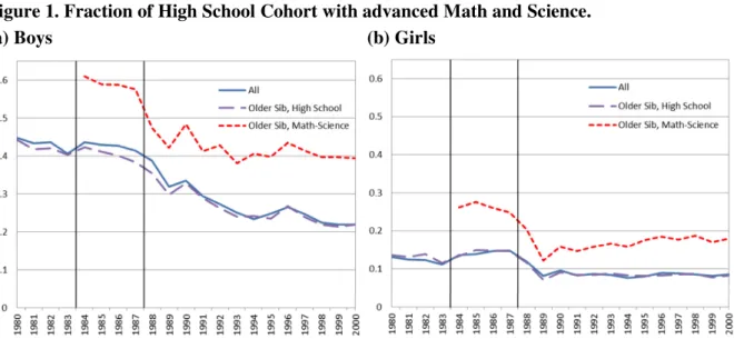
Figure 1 shows the fall in the fraction of the high school cohort who acquired advanced math and science skills over the period 1980-2000 in Denmark. From the figure it is evident that two factors are important: (i) older siblings’ course choices and (ii) school curricula. Those with an older sibling who chose math and science are 14 percentage points more likely to also choose math and science. School curricula were changed at some schools as a part of a pilot scheme in 1984-87 and then they
7
See e.g. Solon (1999) and Black and Devereux (2010) for reviews on intergenerational correlations and Mazumder (2008), Björklund and Salvanes (2010) and Björklund and Jäntti (2012) for sibling correlations.
5
were changed universally in 1988 as part of a reform.8 During the period 1984-87 the falling trend leveled off due to more students choosing math and science at pilot schools. In 1988 a major reform broke up course bundling and gave students (as good as) free course choice, which caused a drop in the number of students opting for math and science. The proportion of girls with math and science stabilized around 8% after 1988, while the gradual decline continued for boys such that only half as many boys chose math and science in 2000 compared to 1980. The gender gap in these advanced skills thus fell by 57% over this 20-year period: from a 31 percentage point difference in 1980 to a 13 percentage point difference in 2000.
Figure 1. Fraction of High School Cohort with advanced Math and Science. (a) Boys (b) Girls
We now specify a model that highlights how the interaction between extrinsic incentives and social multipliers across peer groups may explain this development. The predictions from the model suggest that the time patterns in Figure 1 can be explained by a stronger social multiplier or strong social pressure to conform for boys. A model without intrinsic motivation and social concerns could not explain these patterns without gender-biased changes in preferences or relative skill prices. In our framework, these predictions arise from simply allowing younger sibling’s course choice to depend on the institutional incentives and the choices of their peers. We distinguish between two cases: (a) the older sibling does not choose math-science and (b) the older sibling does choose math-science.
(a) Non-Math-Science older sibling ( 0)
If the older sibling does not choose math-science, the younger sibling’s utility of choosing math-science is given by:
8
6
− − +
(1)
where b denotes extrinsic incentives, which may vary across schools and time; e.g. due to variation in monetary pay, college access, or curriculum design. The term ! + denotes intrinsic costs of
deviating from the choice of the older sibling. The component ! ≡ # $ for
% ∈ '0,1*depends on the older sibling’s course choice whereas the component, , is
unrelated to the older sibling’s particular course choice. ! is the average intrinsic cost for younger siblings who choose differently than their older sibling. This intrinsic cost is the same for everyone in the same peer group, but may vary across peer groups. We define the relevant peer group to be the students in the same cohort at the same school. The primary source of heterogeneity is , which
captures deviations from the average intrinsic cost. ℎ is the truncated mean
over for everyone in the peer group making the same math-science choice. It determines the identity payoff to the relevant course choice.9 We define the gain in identity by conforming with the
older sibling’s choice to be ∆= ℎ = 0 – ℎ = 1 , where
the first term is the pride of conforming with the older sibling and the second term is the prejudice of choosing a math-science identity not conforming with the older sibling.10 is the weight placed on
identity, which may vary with the strength with which social norms are held. Particularly, the weight on identity varies across different peer groups.
The model implies that the younger sibling chooses ℎ = 1 if and only if < ∗ , , , where ∗ , , defines the cut-off below which younger siblings choose advanced Math-Science as a function of extrinsic and intrinsic incentives, and the weight placed on identity. Optimizing younger siblings thus balance the net extrinsic and intrinsic motivation of math-science with the net gains in identity of choosing the same as their older sibling:
− − ∗ , , = ∆# ∗$ (2)
where ∆# ∗$ / | > ∗ 2 – / | < ∗ 2 is the equilibrium gain in identity. We assume that
/ 2 0, which means that∆# ∗$is positive by definition as the first pride-term is positive and the second prejudice-term is negative. The fraction of sibling pairs where the younger sibling chooses math-science and hence does not conform with his or her older sibling is given by
9
Note we choose to use the term identity throughout, but this social factor can be thought of more broadly as a social norm, social reputation, social esteem, or self-image.
10
We choose the terms pride (prejudice) throughout, but they can be interpreted more broadly as honor (stigma) or virtue (guilt). These terms were also adopted by Ellingsen and Johannesson (2008) who provide a related model where some agents have identity concerns and its value depends on the principal. In our model, identity concerns instead depend on the educational choices of the peer group in equilibrium.
7
3 4 ∗# , , $5,11
as those with < ∗ , , choose math-science. We label these non-conformers.
(b)Math-Science older sibling ( ℎ = 1)
If the older sibling chooses math-science then the younger sibling’s utility is given by:
6= ℎ − 1 − ℎ 6 + − ℎ (3)
where 6 + denotes the intrinsic cost of choosing differently than the older sibling. We assume that all other parameters and the distribution of the ex-ante unknown intrinsic cost, , are the same for all younger siblings. Symmetry of the distribution of means that the younger sibling chooses 1 if and only if < 6∗# , 6 , $, where 6∗ , 6 , denotes the cut-off value below which the younger sibling chooses math-science – just like their older sibling. Again the younger sibling balances net gains such that:
+ 6 + ∆# 6∗$ 6∗ , 6 , . (4)
where ∆# 6∗$ / | < 6∗ 2 – / | > 6∗ 2is the equilibrium identity gain from conforming to an older science sibling. Analogously to before, the first term is the pride of choosing math-science like the older sibling and the second term is the prejudice of not conforming. The fraction of sibling pairs where both the younger and older sibling choose math-science is thus given by 3 4 6∗ , 6 , 5. We label these conformers.
From the decision rules (2) and (4) emerges the immediate prediction that younger siblings are more likely to choose math-science if their older siblings chose math-science. As the cut-off is higher when the older sibling chose math-science, 6∗ , 6 , > ∗ , , , it also implies that there are relatively more conformers than non-conformers among the younger siblings choosing math-science,
3 4 6∗ , 6 , 5 > 3 4 ∗ , , 5. This prediction is consistent with the data (presented in detail in
Section 4) and Figure 1: 28% of younger siblings choose math-science conforming to their older sibling, while only 14% are non-conformers and choose math-science even if their older sibling did not. The intuition is that younger siblings receive both extrinsic benefits and additional intrinsic benefits when conforming to their older sibling.
We now turn to the comparative statics and predictions of the model that we will take to the data.
11F
8 2.1. Effects of Extrinsic Incentives
First, we investigate how an increase in extrinsic benefits, b, influences the fraction of younger siblings choosing math-science. The slope of the aggregate math-science supply:
83 4 % ∗ , 9:; % , 5 8 < 4 %∗ , 9:;% , 5 1 1 + 8∆ 4 %∗ , 9:; % , 5 8 ∗ >0 #5$ implies that increasing extrinsic benefits increases the fraction of younger siblings choosing math-science independently of their older sibling’s choice. The last term denotes the social multiplier. The sign of the derivative of conformity, >∆#?∗$
>?∗ , is crucial for whether the social multiplier is above
(below) unity and thus crowds shocks to extrinsic benefits in (out).We can sign the derivative of conformity under mild distributional assumptions.12
Prediction 1.Conformity ∆# ∗$ has a unique interior minimum at ∗ = 0. Thus choices are strategic complements, >∆#?∗$
>?∗ < 0, when MathScience is a rare choice, ∗< 0, while choices are strategic substitutes, >∆#?∗$
>?∗ > 0, when MathScience is a common choice, ∗> 0.
Prediction 1 and (5) thus imply that extrinsic incentives are crowded in by identity when math-science is a rare choice, and crowded out by identity when math-math-science is a common choice. In general, the way the social multiplier reinforces or counteracts shocks to extrinsic incentives across peer groups and schools has implications for math-science choices. Even if all schools are subject to the same curriculum and experience the same curriculum change, they will not experience the same change in the fraction of students choosing math-science. A unique feature of our institutional setting allows us to test Prediction 1 that >∆#?∗$
>?∗ monotonically increases from being negative when
math-science is a rare choice in the peer group to being positive when the choice is more common. That is, when a higher fraction of younger siblings are choosing math-science, there is more crowding out (or less crowding in) via identity concerns. We confront this prediction with data in subsection 2.3. 2.2. Effects of Intrinsic Incentives
Second, we investigate the interaction between intrinsic and extrinsic incentives. The slope of skill supply with respect to the interaction between changes in extrinsic and intrinsic incentives is:
12
9 83 4 % ∗ , 9:; % , 5 8 8 9:;% = 83 4 %∗ , 9:;% , 5 8 8 %∗ 8 %∗ , 9:;% , 8 9:;% #6$ Prediction 2. The interaction effect between extrinsic and intrinsic incentives (6) is negative when MathScience is a rare choice, ∗≪ 0, and positive when MathScience is a common choice, ∗ > 0. Prediction 2 thus implies that a higher intrinsic cost of not conforming counteracts the change in extrinsic incentives when math-science is a rare choice, but reinforces it when math-science is a common choice. 13
2.3. Empirical Evidence of Model Predictions
In this section, we present empirical evidence supporting Predictions 1 and 2. We investigate how course choice responds to changes in extrinsic incentives, b, when math-science is a rare choice and a common choice, respectively. We measure the fall in extrinsic incentives by the indicator, B/ ≥ 19882, which measures how the choice set was universally and uniformly changed for all high school cohorts entering high school after 1988.
To investigate the empirical support for Prediction 1, we compute the fraction of school-cohort-mates’ older siblings choosing math-science: GGGGGGGGGGGGGGGGGℎ F ,H,I, where s denotes high school and t denotes cohort of the younger sibling.14 Figure 2 presents difference-in-differences coefficient estimates, αε∗ , on the interaction between whether this fraction is higher than a cut-off value, ∗, and the reform indicator: B GGGGGGGGGGGGGGGGGℎ F ,H,I ≥ ∗ ∗ B/ ≥ 19882 plotted against the cut-off, ∗.The regression also controls for whether the younger sibling enters high school after the major reform in 1988, B/ ≥ 19882, high school Pilot status, high school fixed effects, and cohort fixed effects. Each regression coefficient, αε∗, thus measures the difference in the impact of the (negative) shock to
extrinsic incentives between high schools above and below the cut-off, ∗. Varying the cut-off in Figure 2 from low (0.05) to high (0.5) thus shows the impact of the (negative) shock depending on how rare or common math-science is in the peer group. The reform caused a large decline in the fraction of students choosing math-science. It was essentially a decrease in extrinsic incentives as it signaled less importance to bundling these advanced courses. That is, a positive regression coefficient, αε∗> 0, means a negative derivative, >∆#?
∗$
>?∗ < 0, of identity gain. 13
See Appendix A for more details and derivation of Prediction 2.
14
We get very similar results if we instead proxy the peer group norm by the fraction of school-cohort-mates’ older siblings at a Pilot school or by the fraction of school-cohort-mates’ parents with a STEM education.
10
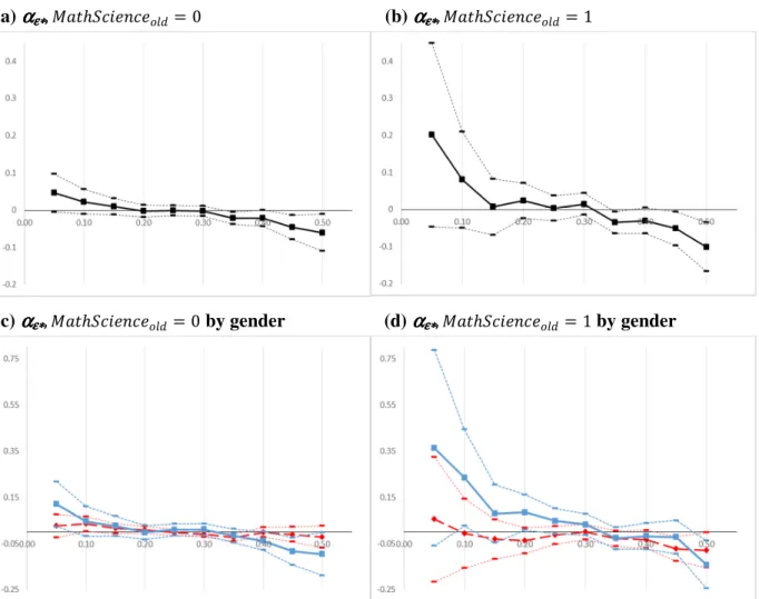
Figure 2 shows how the derivative >∆#?>?∗∗$goes from being negative when math-science is a rare choice in the peer group to being positive when it is a more common choice. Furthermore, a comparison of panels (a) and (b) shows a steeper slope when the older sibling chose math-science. This means that the change in the social multiplier is larger and there is more crowding in of the weaker extrinsic incentives for the younger siblings who would previously conform to their older sibling by choosing math-science. In a model without intrinsic motivation and identity concerns, we would expect identical individuals to respond identically to a universal curricula change independently of their peer group (i.e. horizontal curves).
Figure 2. Crowding in of Extrinsic Incentives.
(a) ααααε∗ε∗ε∗ε∗, ℎ 9:;= 0 (b) ααααε∗ε∗ε∗ε∗, ℎ 9:;= 1
(c) ααααε∗ε∗ε∗ε∗, ℎ 9:;= 0 by gender (d) ααααε∗ε∗ε∗ε∗, ℎ 9:;= 1by gender
Note: The figure displays the regression coefficient, αε∗, and 95% confidence intervals (vertical axis) by the fraction of
school-cohort-mates’ older siblings with math-science, GGGGGGGGGGGGGGGGGℎ F ,H,I (horizontal axis) as a proxy for the variation in the cut-off value, ∗, for whether younger siblings are indifferent between choosing math-science or not. All estimates are displayed separately by older siblings’ math-science choice and by gender in panels (c) and (d), where the light solid line with squares denotes boys and the dark dashed line with diamonds denotes girls.
11
To investigate the empirical support for Prediction 2 we also need exogenous variation in intrinsic incentives. In this section, we provide suggestive evidence based on the observation that cut-offs vary by gender. In sections 5 and 6 we further exploit the pilot scheme shifting the math-science choice of the older sibling and thus shocking the younger sibling’s intrinsic cost of not conforming.
Our data reveals that the gender of the older sibling seems to matter for younger sisters, as 21% conform to an older sister while only 14% conform to an older brother, whereas 42% of younger brothers are conformers, independently of their older sibling’s gender.15 These patterns might suggest that the intrinsic costs of not conforming are higher for boys than for girls. Therefore, we distinguish between genders of younger siblings in panels (c) and (d) in Figure 2. The slope is steeper for younger brothers than for younger sisters suggesting that there is stronger crowding in for younger brothers than for younger sisters. Furthermore, the total drop in math-science skill supply after the 1988 reform is 8.7 percentage points larger for boys than for girls.16 If we accept that boys face higher costs of not confirming, these observations are in line with Prediction 2. It is well-known in the literature that gender is a salient part of identity and that math-science choices vary by gender, therefore the model also implies that the identity concerns in course choice likely vary by gender. 17 We believe the above results relate to gender stereotypes of math-science meaning that boys face a stronger social pressure to conform as math and science are stereotypical male choices.18 This is also consistent with Joensen and Nielsen (2014) who find that the baseline monetary payoff for the marginal girl to choose advanced math and science is substantial when only 20% of girls in the high school cohort are choosing it, while it is lower (approaching zero) for the marginal boy when more than 50% of boys choose advanced math and science.
Overall, this section substantiates how the interplay between changes in extrinsic incentives and changes in intrinsic costs and social norms across peer groups may have contributed to the continuous fall in the math-science supply. Over the period 1980-2000, this advanced skill supply has decreased by 50% among boys and the gender gap has closed by 57% as the social pressure to take advanced math and science in high school, which seem to have been particularly strong for
15
The numbers referred to may be found in Figure A1 in Appendix A and Table B3 in Appendix B.
16
This is concluded by replacing the cut-off proxy, B GGGGGGGGGGGGGGGGGℎ F ,H,I≥ ∗ , in the Figure 2 regressions with a male indicator variable.
17
See e.g. Akerlof and Kranton (2002), Bertrand (2010), and Bertrand et al. (2013) for evidence on gender identity. See e.g. Joensen and Nielsen (2014) and Buser, Niederle and Oosterbeek (2014) for evidence on gender differences in math-science high school course choices.
18
12
boys, was loosened up. Thus implementing a curriculum signaling less importance of combining advanced math and science leads to a larger drop in math-science skill supply for boys than for girls.
In order to better understand why we observe more crowding in for boys, we turn to estimating causal sibling spillover effects. These are essential for understanding how strongly social multipliers may amplify or dampen impacts of education policies depending on the composition of the peer group. We exploit the fact that the pilot scheme shocked younger siblings’ intrinsic incentives indirectly by shocking their older siblings’ extrinsic incentives, while the 1988 reform changed their extrinsic incentives directly. We thus assess the magnitude of this interaction effect by examining younger siblings’ math-science choices and how they are affected by the social interaction effects with their older siblings. Testing Prediction 2 requires enough variation in how rare and common the math-science choice is, which we have because of the phase-in of the pilot-scheme in place for the older siblings who entered high school during the pre-reform years 1984-87.19 The following two
sections lay out the identification strategy, institutional details, and the data, while sections 5 and 6 are devoted to analyzing these mechanisms in detail.
3.
Identification of Peer Effects Using a High School Pilot Scheme
We exploit some unique features and changes in institutions in Denmark to identify the peer effects in sibling interactions. This section describes our identification strategy and the educational environment of the Danish high school. In the first subsection, we briefly explain the empirical challenge of identifying peer effects and how we exploit the unique institutional setup to identify social interaction effects from older to younger siblings. Then we describe the two relevant high school regimes, which form the basis for our identification strategy. The second and third subsections, concern the high school regime and the pilot scheme that provides us with exogenous variation in the cost of acquiring advanced math and science courses for the older siblings. The fourth subsection, concerns the high school regime forming the basis for the math and science choices of their younger siblings.
19
Jia and Persson (2014) present a similar model to explain child identity choices of minority couples in China. They primarily exploit exogenous time-series variation in extrinsic incentives induced by the one-child policy, but do not have enough exogenous variation shifting the cut-off in the cross-section and rely on regional variation instead. In this subsection we rely on similar time and cross-sectional variation across high schools caused by the policy changes detailed in Section 3, while we even exploit exogenous variation in the cut-offs in the cross-section in Section 5 and 6.
13 3.1. Identifying Peer Effects
Peer (or social interaction) effects occur when the choice of one individual affects the choices of other individuals in the same peer (or social) group. In this paper, we are interested in how math and science choices of an older sibling affect whether his or her younger sibling pursues advanced math and science courses. The general challenge of identifying peer effects lies in the empirical issues of: (i) endogenous group membership, (ii) simultaneity (the reflection problem), and (iii) correlated unobservables in the peer group.20 These identification issues can be illustrated in a model which is linear in the peer effect. We assume, without loss of generality, that there are only two individuals in each peer group - an older sibling and a younger sibling.21
ℎ = K + K6 ℎ + KLM + KNM + KO P+ ,P (7)
Q + Q6 + QLM + QNM + QO P+ ,P (8)
where R denotes whether sibling i chose advanced math with an advanced science course in high school, MR denotes observable characteristics of sibling i, P denotes sibling pair specific characteristics like family background, gender composition, and age difference. Finally, R,P denotes other unobserved factors affecting the MathScience choice of individual i in sibling pair f.
Our objective is to estimate a causal effect of the older sibling’s choice on the
younger sibling’s choice. To be able to give a causal interpretation of the
parameter estimate of Q6 in (8) we need to address the empirical issues (i)-(iii) mentioned above. The third issue of correlated unobservables is naturally a big concern in our setting, since siblings share many common social and genetic influences; including common genes, family background, neighborhood, and schools. All these common influences shape both siblings’ preferences and abilities and could lead them to making similar high school course choices. Omitted variables bias due to contextual effects arises if we are not able to observe all these relevant sibling pair specific ( P) and individual variables (MR). The first and the second issues are presumably minor in our setting: (i) siblings are born into the same family thus do not choose each other based on each other’s characteristics and choices, and (ii) given the timing of high school course choices it seems plausible that the older sibling’s course choice is independent of the younger sibling’s choice (K6 0) since
20
Manski (1993; 1995) provides a more complete and general analysis of the identification of peer effects (or more generally endogenous effects), while Moffitt (2001) introduces the conceptual framework we adopt here. In a more recent contribution, Angrist (2014) discusses the identification challenges.
21
It is straightforward to generalize this setting to larger peer groups. Brock and Durlauf (2001) discuss identification in nonlinear peer effects models.
14
the older sibling makes this choice years before the younger sibling. This exclusion restriction overcomes the reflection problem, as we postulate that the direction of the sibling effect goes from the older sibling to the younger sibling.22 Nevertheless, this is not a necessary exclusion restriction as our empirical strategy addresses all these three empirical concerns, since the exogenous variation in the cost of acquiring advanced math and science for the older sibling is independent of both sibling pair specific factors and individual sibling characteristics.
More specifically, our identification strategy exploits exogenous variation in the cost of acquiring advanced math and science stemming from a pilot scheme, where some older siblings unexpectedly got the option of a more flexible course combination. Let S :9 B T9 0 for older siblings in a traditional high school, where advanced math and science could only be achieved in a package of advanced math, advanced physics and intermediate chemistry. Let S :9 B T9 = 1 for older siblings in a pilot high school, where advanced math and science could also be achieved in a package of advanced math, advanced chemistry, and intermediate physics. This additional course package option was introduced unexpectedly just before the older sibling made the choice of advanced high school courses. The pilot scheme thus provides us with exogenous variation in the cost of acquiring advanced math and science for the older sibling (captured by S :9 B T9 ) that does not directly influence the younger sibling and is independent of any sibling pair specific ( P) and individual variables (MR). Substituting this into (9) and (10) we get:
ℎ = K + US :9 B T9 + KLM + KNM + KO P+ ,P (9)
Q + Q6 + QLM + QNM + QO P+ ,P (10)
Younger siblings attend high school in a regime, where they have an even more flexible curriculum as advanced math and science courses can be combined as they like - the main requirement is that they choose at least two (and at most three) optional advanced courses. This particular institutional setting thus provides us with a unique quasi-experiment for identifying peer effects in math and science - going from the older sibling’s course choice to the younger sibling’s course choice. We can thus interpret the IV estimate of Q6 in the structural equation (10) as capturing this causal peer effect
when the first-stage equation (9) includes S :9 B T9 as an instrument for which
endogenously affects , because the instrument only affects the older sibling
22
The developmental psychology literature supports that the direction of behavioral influence goes from the older sibling to the younger sibling (Buhrmester, 1992). Altonji et. al (2013) also corroborate this assumption and impose it as an identifying assumption to estimate causal sibling influences on adolescence substance use.
15
directly and the younger one merely through endogenous social interaction.23 The identifying assumptions are corroborated in Joensen and Nielsen (2009, 2014) showing that S :9 B T9 is independent of predetermined individual, family, and school characteristics for the students entering high school in 1984-87. This implies that older siblings are as good as randomly assigned to high schools which unexpectedly introduce the pilot scheme when they are enrolled in their second high school year. Subsection 3.3 provides additional tests to corroborate instrument validity in this setting. Furthermore, the instrument has a strong influence on the choice of math and science courses for the older sibling. We return to these empirical issues in Section 5. The following subsections describe the educational environment of the two relevant high school regimes: The Pre-1988 High School with restrictive course packages that the older siblings attended and the Post-1988 High School with much more flexible course choices for their younger siblings.
3.2. The Pre-1988 High School
In the period 1961-1988, the Danish high school system was a "branch-based" high school regime in which courses were bundled into restrictive course packages.24 We focus on the cohorts entering high school in 1984-87. The main reason to focus on this period is that the supply of course packages provides us with relevant exogenous variation in the cost of acquiring advanced math and science for the older siblings.
This regime implied that students upon high school graduation would have achieved one of three math levels available: advanced, intermediate, or basic level. The difference between the three levels is reflected in the number of lessons per week, as well as in the content of the courses. For instance, the extent of geometry and algebra increases as the level becomes more advanced. In the empirical analysis, we focus on whether students choose advanced math and science, meaning that the intermediate and basic level courses are lumped together. The decision about which package to opt for is taken at the end of the first year in high school. The only way to obtain advanced math and science was the package consisting of advanced math, advanced physics and intermediate chemistry, unless the student was enrolled at a pilot school, where the package could be adjusted to include advanced chemistry and intermediate physics instead. It is exactly this increased course flexibility
23
Moffitt (2001) labels this type of identification strategy as a partial-population policy intervention.
24
Available course packages were labelled: Social Science and Languages, Music and Languages, Modern Languages, Classical Languages, Math-Social Science, Math-Natural Science, Math-Music, Math-Physics, and Math-Chemistry. The additional course package introduced at pilot schools was the Math-Chemistry option.
16
which some students were unexpectedly exposed to that constitutes the quasi-experiment we exploit in this paper.
3.3. The Pilot Scheme
The pilot scheme was implemented as an experimental curriculum at about half of the high schools prior to the 1988-reform. The purpose of the pilot scheme was to test the impact of increased flexibility prior to the 1988-reform. Figure 3 illustrates the consequences of the pilot scheme on the course packages of the high school youth. Prior to the pilot scheme, the fraction choosing advanced math and science declined and went below 25% in 1983. The pilot scheme counteracted this declining trend by attracting youth to the alternative course package with a higher weight on chemistry and a lower weight on physics.
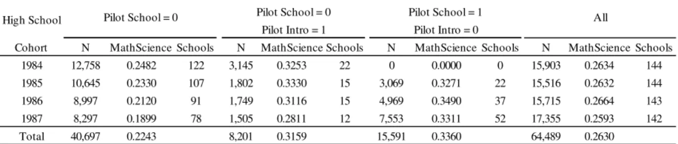
Table 1 gives an overview of the gradual implementation of the pilot scheme from 1984-87. The table is divided by types of high schools: schools with no pilot scheme (PilotSchool=0), schools where the pilot scheme was introduced after enrollment of the relevant cohort (PilotSchool=0, PilotIntro=1), and schools where the pilot scheme was implemented prior to enrollment of the relevant cohort (PilotSchool=1,PilotIntro=0).
Figure 3. Fraction of High School Cohorts Choosing Math-Science, by School Type
Note: Pilot schools include all schools with pilot status at any point in time during 1984-87; i.e. 64 schools in total. 0.00 0.05 0.10 0.15 0.20 0.25 0.30 0.35 1 9 8 0 1 9 8 1 1 9 8 2 1 9 8 3 1 9 8 4 1 9 8 5 1 9 8 6 1 9 8 7 1 9 8 8 1 9 8 9 1 9 9 0 1 9 9 1 1 9 9 2 1 9 9 3 1 9 9 4 1 9 9 5 1 9 9 6 1 9 9 7 1 9 9 8 1 9 9 9 2 0 0 0 Pilot School
17
Schools were not randomly assigned to become pilot schools, but we provide evidence that assignment was as good as random. From 1984-86, schools could apply to the Ministry of Education for permission to adopt the experimental curriculum, whereas in 1987 the high school principals could make this decision without approval from the ministry.25 It is not possible to directly test whether the pilot schools represent a sample of schools which is essentially random with respect to math and science ability, but we corroborate that this is a reasonable assumption.
It is clear, however, that students with a particular preference for chemistry may self-select into schools that are known to offer the pilot program before entrance. This is why we distinguish between students at pilot schools where the pilot scheme was unexpectedly introduced after they had enrolled (PilotSchool=0, PilotIntro=1) and those who knew that the school was a pilot school before they applied for entering the school (PilotSchool=1, PilotIntro=0).
Table 1. Introduction of the Pilot Scheme
Note: The table illustrates the introduction of the pilot scheme. For each of the affected cohorts, 1984-86, the table displays the number of schools who are traditional high schools only offering advanced Math with advanced Physics (PilotSchool=0), who are unexpectedly introducing the pilot scheme combining advanced Math with advanced Chemistry (PilotSchool=0, PilotIntro=1) and who already have adopted the pilot scheme (PilotSchool=1, PilotIntro=0).
The instrumental variable strategy exploits the fact that the pilot scheme reduces the psychological cost of choosing advanced math and science since the students exposed to the scheme are free to choose either advanced physics and intermediate chemistry or advanced chemistry and intermediate physics.26 Hence, first-year high school students enrolled at a school when it decided to introduce the pilot scheme were exposed to an unexpected exogenous cost shock, which induced more students to choose advanced math and science compared to students at non-pilot schools. If the selection of
25
The schools which introduced the program in 1987 tend to be slightly negatively selected in terms of the students’ math abilities, while no similar concerns are raised regarding the other cohorts. However, to maintain a large number of sibling pairs, we include the 1987 cohort of older siblings in the study, while checking the sensitivity of our results to leaving out this cohort.
26
Traditionally, the opportunity cost of attending high school is interpreted as forgone earnings from unskilled work. We use a broader interpretation associated with time allocation across courses as well as between studies, leisure, and unskilled work. If students choose course combinations optimally given their preferences and abilities, then a more flexible choice set reduces the cost of taking a given course as there is a higher probability of a good match between feasible course combinations and the students' preferences and abilities.
Cohort N MathScience Schools N MathScience Schools N MathScience Schools N MathScience Schools
1984 12,758 0.2482 122 3,145 0.3253 22 0 0.0000 0 15,903 0.2634 144
1985 10,645 0.2330 107 1,802 0.3330 15 3,069 0.3271 22 15,516 0.2632 144
1986 8,997 0.2120 91 1,749 0.3116 15 4,969 0.3490 37 15,715 0.2664 143
1987 8,297 0.1899 78 1,505 0.2811 12 7,553 0.3311 52 17,355 0.2593 142
Total 40,697 0.2243 8,201 0.3159 15,591 0.3360 64,489 0.2630
Pilot School = 0 Pilot School = 0 Pilot School = 1 All
High School
18
newly participating schools is exogenous with respect to student ability, the pilot scheme provides exogenous variation in students' math and science skills without influencing the outcome(s) of interest except through the effect on math and science choices.
The instrumental variable, PilotIntro, is equal to one if the individual enrolled in a high school which then introduces the experimental curriculum for the first time, and it takes the value zero otherwise. This instrument is valid if the pilot scheme is randomly assigned to schools and if individuals are randomly distributed across schools that have not yet decided to introduce the experimental curriculum. This assumption is violated if the school decides to participate in the program based on the math abilities of local students. In Section 4 below, we test for similarities of student and parent characteristics across school status, and we find almost no significant differences in characteristics determined prior to high school. The assumption is also violated if schools change as a consequence of the scheme: if the school develops an expertise in science or if the quality of teachers changes as a consequence of the pilot scheme. Such effects would influence the younger siblings if they attend the same high school as their older siblings, and the effects could confound the sibling peer effects. However, Figures 1 and 3 showed that the pilot scheme was introduced following a declining trend in the fraction choosing advanced math and science, and therefore qualified teachers would most likely be available. Furthermore, the relevant compliers would switch from intermediate chemistry and intermediate math to advanced chemistry and advanced math which would require only 5-6 additional weekly lectures for one class per cohort per school.
In the empirical analysis we investigate to what extent the spillover effects may be going through the high school rather than through sibling interactions. We find that the bulk (at least 60%) of the spillover effect goes through social interactions among siblings.
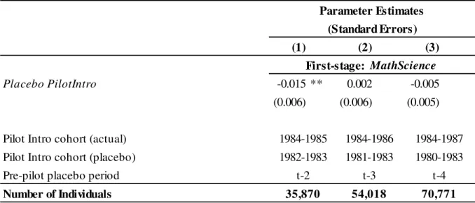
Table 2 presents placebo tests to support instrument exogeneity. The table presents first-stage estimates (falsely) assuming that the pilot scheme was introduced two, three, or four years, respectively, prior to when it was actually introduced. The first specification assumes that the pilot scheme was implemented for the cohorts who were in their third and final year when the pilot was actually adopted, while the last two specifications assume that it was implemented for recently graduated cohorts. Neither of these cohorts should be affected, since they should already have made their final course choices before the pilot scheme was adopted. We find a small significantly negative effect of the pilot schemes for the first placebo test. This suggests that the schools introducing the pilot in 1984-85 had slightly (1.5 percentage points) fewer students choosing math and science before the school adopted the pilot program. The coefficient is small and the picture is consistent with what is also seen in Figure 3. However, in the two last specifications where the distance to the
19
actual reform is longer, the effect is smaller and insignificant. We therefore conclude that there existed only minor, if any, systematic prior differences in choices at schools which adopted the pilot scheme, and if anything, they should work in the opposite direction of the pilot.
The instrument is strong if the unexpected introduction of the pilot scheme induces students to choose advanced math and science, which is directly tested and validated in Section 4. The instrument satisfies the monotonicity (or uniformity) condition if individuals who chose advanced math and science when required to do advanced physics and intermediate chemistry would also have chosen advanced math and science if they unexpectedly got the option of replacing advanced physics with advanced chemistry and replacing intermediate chemistry with intermediate physics. We are confident that the monotonicity assumption is reasonable in our application, since all options available at non-pilot schools were also available at schools introducing the pilot scheme.
Our instrument exploits the exogenous variation in the exposure of students to the option of switching the levels of physics and chemistry. Hence, the treatment of the older sibling that we investigate is the combined treatment of advanced math with advanced chemistry and intermediate physics. We cannot separately identify the effect of math and science courses from the potential synergy between them.
Table 2. Placebo Tests on Pre-Pilot Cohorts
Note: Parameter estimates and (standard errors) of the placebo pilot scheme introduction are displayed for first-stage OLS regressions of MathScience choice. The columns differ in which cohorts the placebo pilot introduction is assumed for and which schools are included in the sample. Column (1) leads PilotIntro two cohorts by assuming it was implemented for those who are graduating from the relevant school in the year it was actually implemented. Columns (2) and (3) lead PilotIntro three and four cohorts, respectively, by assuming it was implemented for those who have already graduated from the relevant school in the year it was actually implemented. The full set of cohort and parental background control variables is included. Significance at a 1%-, 5%-level and 10%-level are indicated by ***, ** and *, respectively.
(1) (2) (3)
Placebo PilotIntro -0.015 ** 0.002 -0.005
(0.006) (0.006) (0.005)
Pilot Intro cohort (actual) Pilot Intro cohort (placebo) Pre-pilot placebo period Number of Individuals Parameter Estimates (Standard Errors) First-stage: MathScience 1984-1985 1984-1986 1984-1987 35,870 54,018 70,771 1982-1983 1981-1983 1980-1983 t-2 t-3 t-4
20
3.4. The Post-1988 High School
In 1988 there was an extensive structural reform of the Danish High School, which was the most fundamental high school reform since 1903. The reform abolished the “branch based” regime and substituted it with a “choice based” regime, where the main distinction is between mathematical and linguistic track students. The reform implied an extended choice set in the form of more flexible opportunities to combine optional courses.27 In particular, the mathematical track students have the option of combining advanced math with any other advanced course; for example physics, chemistry, biology, social science, or a language course. This is the regime within which the younger siblings in our sample make their educational choices. We focus on the younger siblings’ choice of advanced math with advanced physics and/or advanced chemistry, since these are comparable to the relevant course combinations for the older sibling attending high school in the pre-1988 regime.
In the post-1988 high school regime, students choose either the mathematical or the linguistic track upon entry. Each course is either common to all students on the chosen track (compulsory courses), compulsory for some and optional for others, or exclusively optional. The optional courses can be obtained at either advanced or intermediate level reflecting the complexity of the content, the number of lessons per week and the intensity of exams (written and/or oral).
All students are required to follow at least two (and at most three) optional advanced courses, and for the mathematical students there was a minimum required amount of math-science content, while for the linguistic students there was a minimum required amount of language content. The first year of high school consists only of compulsory courses (common as well as track-specific courses) taught in classes of at most 28 students. The second and third year of high school added at least three and at most four optional courses.28. In addition to the requirements of at least two advanced optional courses, there were some bonds between some courses in order to preserve the possibility for the courses to complement each other.
27
The reform also implied more weight on the high schools’ role of preparing students for college, more required readings, more written assignments, more stringent non-attendance regulation, more grading, and more hours of instruction allocated to the compulsory courses.
28
The compulsory courses common to all students are advanced Danish and history, intermediate English and basic physical education, biology, geography, religion, music, (visual) art, and ancient history. Track-specific compulsory courses for mathematical students comprise intermediate math and physics, basic chemistry, and a second foreign language. For the linguistic students the track-specific compulsory courses are basic natural sciences (including math) and Latin, as well as two other foreign languages. Commonly available optional intermediate courses comprise: biology, geography, chemistry, technical science, business and economics, drama, sports, and movie science, while optional advanced courses include all feasible continuations of the intermediate courses.
21
We follow younger siblings in this high school regime until the entry cohort of 1997. We focus on the younger siblings’ choice of advanced math with either advanced physics or advanced chemistry, since these are comparable to the relevant pre-1988 regime course combinations of the older siblings.29 Thus in equation (7) is an indicator for whether the younger sibling chooses to combine advanced math with either advanced physics or advanced chemistry.
4.
Data Description
4.1. Sample Selection
For our empirical analysis we use a panel data set comprising the population of individuals starting high school from 1984 and onwards. The data are gathered from administrative registers and administered by Statistics Denmark. The data include basic demographic information such as date of birth, place of residence, and gender. What is crucial for this study is that we observe which schools offered the pilot scheme when, and we can identify which school the individual attended as well as the chosen course package. Furthermore, we have information about the dates for entering and exiting a high school education, along with an indication of whether the individual completed the education successfully, dropped out, or is still enrolled as a student. We augment this data with background information about the parents; including educational achievement and gross income. This information is recorded when the individual was 15-years old, which is prior to enrolling in high school.
The sample consists of individuals who are directly influenced by the quasi-experimental variation due to the gradual introduction of the pilot scheme for cohorts entering high school 1984-1987. From this sample, we select high school graduates who finished in three years and have a younger sibling who entered high school after 1987 and finished in three years.30 In our main analysis, we focus on a homogeneous sample of relatively closely spaced sibling pairs (cohorts 1988-91, age gap ≤ 4 years).31
29
Some curriculum changes are introduced with the reform, e.g. a historical dimension was incorporated into the math course while some advances in the experimental direction were incorporated into the physics course.
30
About 40% of a birth cohort attended the academic high school track at this point in time; hereof 10% do not complete in three years. The main part of drop out takes place before the choice of advanced math and science course packages. For older as well as younger siblings, dropout is uncorrelated with pilot school status.
31
An overview of the sample selection is given in Table B1 in Appendix B. An overview of the distribution of sibling pairs across the older siblings’ exposure to the pilot scheme for each high school cohort of younger siblings is given in Table B2 in Appendix B.
22
4.2. Outcome and Control Variables
The outcome of interest is whether the post-reform peers choose to combine advanced math and science or not. Table B3 reveals a strong correlation in the choice of this course package across siblings: 28 % (14 %) of younger siblings chose this course package when the older sibling did (did not) choose this package, and the correlation varies across gender composition of the sibship.
Table B4 shows variation in the choice of advanced math and science when we distinguish between whether the older sibling was exposed to the pilot scheme or not. The proportion of younger siblings who chose this course package is 18% when the older sibling was not exposed (PilotSchool=0, PilotIntro=0) and 22% when the older sibling was unexpectedly exposed to the pilot scheme (PilotSchool=0, PilotIntro=1). The relationship appears to be very strong among pairs of brothers.
We also include entry cohort fixed effects, sibling gender composition, parental background, and high school specific controls. Parental background includes a set of mutually exclusive indicator variables for the level of highest completed education of the mother and father, respectively, and their income as observed at the end of the year before the individual started high school.
Table B5 in Appendix B shows descriptive statistics of background variables across pilot school status. From this table it is evident that the students whose older siblings entered high schools which had already adopted the pilot program (PilotSchool=1, PilotIntro=0) previous to their entry are potentially non-randomly selected, while those whose older siblings were unexpectedly exposed to the program (PilotSchool=0, PilotIntro=1) are not systematically different from students at schools without the pilot program (PilotSchool=0, PilotIntro=0). This lends further support for the validity of PilotIntro as an instrument for older siblings’ course package choice.
5.
Estimates of Sibling Peer Effects
Table 3 presents the main results from the empirical analysis of how an increase in extrinsic incentives for the older sibling spill over on their younger sibling through increasing their intrinsic motivation. We present the results from OLS and 2SLS while the main results are similar for alternative methods.32 The OLS regressions indicate a strong positive association between math and
32
We report the results from the bivariate probit estimator in Table B6 in Appendix B. Our main results are robust and the first-stages are literally unchanged. Conclusions from the bivariate probit model appear slightly stronger; particularly in the subgroup analysis. However, as in Altonji, Elder and Taber (2005) identification is mainly driven by the parametric assumptions when covariates are included in the bivariate probit model. In addition, we have used the
23
science course choices of older and younger siblings. The reduced form estimates suggest that there are spillover effects from the introduction of the pilot scheme onto the younger siblings, while the IV estimates suggest that the effect goes through the older siblings’ course choices. However, the effects are only statistically significant when the age distance between the siblings is less than four years.33 When the age distance is less than four years, the magnitude of the estimates ranges from 0.35-0.52, which suggests a very strong peer effect.
Including additional control variables does not significantly affect the point estimates, lending additional support to the exclusion restriction and exogeneity of PilotIntro which is imperative for the causal inference based on the IV estimates. Columns (3) and (6) add explanatory variables related to high schools: an indicator variable for whether the siblings attended the same high school and predetermined high school means of parents’ highest completed education and income. These mean variables are thought to approximate permanent high school specific effects such as the quality of science teachers or the expertise in science teaching. In Table B8 in Appendix B we further investigate whether the spillover works through the school rather than the sibling. We present results from a placebo test where we randomly match only children from entry cohorts 1984-87 with only children from entry cohorts 1988-91. At the left hand side of the table we match the children randomly and at the right hand side we randomly match only children attending the same high school. No matter how we match the children, there is no correlation between their course choices. When we match only children attending the same high schools, the reduced-form coefficient and the 2SLS coefficients are larger than when they are randomly matched. However, the estimates are 40% smaller compared to the main results in Table 3 and insignificant. When high school specific variables are added (columns (6) and (8)) they are even smaller. We conclude that it is important to account for the high school specific variables in order to rule out that the spillover effect goes through the school.34
semi-parametric estimator by Abadie (2003) as a robustness check. The second stage estimate without control variables is statistically indistinguishable from the bivariate probit (marginal effect 0.384 vs. 0.360).
33
Table B7 in Appendix B presents the results when the maximum age difference is held constant and the cohorts are allowed to vary. These results confirm that the results vary with age difference and not with cohorts. This is consistent with sibling pairs with an age difference of five years or more being considers separate sibships (Adams, 1972).
34
It should be noted that only children attending the same high school may know each other and socially interact through extra-curricular activities like sports clubs. This direct social interaction is less likely if their age difference is larger. When we leave out the placebo siblings within the same high school with an age difference of less than two years, then the unconditional reduced form coefficient in (5) further falls to insignificant 0.014. Likewise, the 2SLS estimate is also insignificant and 60% smaller compared to our main estimates in Table 3.
24
Table 3. Estimates of Peer Effects: Main Results
Note: Significance at a 1%, 5%, and 10% level are denoted by ***, ** and *, respectively.
N (1) (2) (3) (4) (5) (6) PilotIntro 0.068 *** 0.071 *** 0.065 *** Younger Sibling 1988-91, ≤4y 7,786 (0.017) (0.016) (0.017) PilotIntro 0.065 *** 0.070 *** 0.067 *** Younger Sibling 1988-92, ≤5y 10,571 (0.015) (0.014) (0.014) PilotIntro 0.060 *** 0.067 *** 0.063 *** Younger Sibling 1988-93, ≤6y 12,717 (0.013) (0.013) (0.013) PilotIntro 0.067 *** 0.073 *** 0.069 ***
Younger Sibling 1988-97, ≤10y 17,691 (0.011) (0.010) (0.011)
PilotIntro 0.036 ** 0.032 ** 0.023 Younger Sibling 1988-91, ≤4y (0.015) (0.014) (0.014) PilotIntro 0.020 * 0.017 0.01 Younger Sibling 1988-92, ≤5y (0.012) (0.012) (0.012) PilotIntro 0.017 0.013 0.067 Younger Sibling 1988-93, ≤6y (0.011) (0.011) (0.011) PilotIntro 0.010 0.009 0.006
Younger Sibling 1988-97, ≤10y (0.009) (0.009) (0.009)
Older Sibling MathScience 0.140 *** 0.147 *** 0.145 *** 0.523 ** 0.447 ** 0.346
Younger Sibling 1988-91, ≤4y (0.009) (0.010) (0.010) (0.231) (0.205) (0.221)
Older Sibling MathScience 0.145 *** 0.151 *** 0.150 *** 0.314 0.241 0.149
Younger Sibling 1988-92, ≤5y (0.008) (0.008) (0.008) (0.192) (0.168) (0.177)
Older Sibling MathScience 0.142 *** 0.149 *** 0.147 *** 0.276 0.193 0.106
Younger Sibling 1988-93, ≤6y (0.007) (0.007) (0.007) (0.183) (0.155) (0.168)
Older Sibling MathScience 0.139 *** 0.146 *** 0.144