Archive of SID. Frequency Analysis of a Cable with Variable Tension and Variable Rotational Speed.

Archive of SID

Frequency Analysis of a Cable

with Variable Tension and

Variable Rotational Speed

Moharam Habibnejad Korayem*

Department of Mechanical Engineering,

Iran University of Science and Technology, Tehran, Iran E-mail: [email protected]

*Corresponding author

Ali Akbar Alipour

Department of Mechanical Engineering,

Iran University of Science and Technology, Tehran, Iran E-mail: [email protected]

Received 19 June 2011; Revised 12 August 2011; Accepted 01 September 2011

Abstract: In this paper coupled nonlinear equations of motion of a suspended

cable with time dependent tension and velocity are derived by using Hamilton’s principal. A modal analysis for a stationary sagged cable is initially carried out in order to identify the dynamic system. The natural solution is directed to compute the natural frequencies and mode shapes of the free vibration of a suspended cable. Natural frequencies and mode shapes are plotted versus a dimensionless parameter

λ, known as static sag character. In case of moving cable, the tension force and the

rotary speed of the pullies are assumed to be sinusoidal functions. Galerkin mode summation approach is utilized to discretize the nonlinear equations of motions. Numerical simulations are carried out in the time domain. A frequency analysis is then carried out and effects of the frequency of tension force and rotary speed on the belt dynamic responses are studied.

Keywords: Cable, Frequency Analysis, Galerkin’s Method, Nonlinear Vibration,

Parametric Study.

Reference: M. H. Korayem and A. A. Alipour, (2011) ‘Frequency Analysis of a

Cable with Variable Tension and Variable Rotational Speed’, Majlesi Journal of Mechanical Engineering, Vol. 4/No. 4, pp. 1-8.

Biographical notes: M. H. Korayem received his PhD in Mechanical

Engineering from University of Wollongong, Australia 1994. He is currently full Professor at the Department of Mechanical Engineering, Iran University of Science and Technology, Tehran. His current research interest includes Modeling,

Simulation and Design of Industrial Robots. A. A. Alipour received his B. Sc. in

Mechanical Engineering. He has also obtained his master's degrees in Mechanical Engineering at the Iran University of Science and Technology. He is interested a Suspended Cable.

Archive of SID

1 INTRODUCTION

The free vibration analysis of a suspended cable has attracted much of interest in engineering mechanics especially in last decades. The vibration of many important engineering structures such as overhead transmission lines, gay cables and tracks can be represented using the suspended cable model. In practice the actual oscillations occurring in cables depend on static sag due to the cable weight. It can be shown that due to this static sag, the longitudinal and transversal modes of vibration are coupled and equations of motions become fully nonlinear.

Irvin’s theory [1] was the first theory, presented in this context. According to this theory eigenvalues and eigenfunctions of differential equations of motion can be calculated using an appropriate numerical method while neglecting non-linear terms. This theory is also presented in [2]. In [3] differential equations of motion are solved using the method of separation of variables and also by another numerical method. In [4], natural frequencies and mode shapes of a suspended cable are computed using finite element method.

Free vibration analysis of a track, which is simulated with a suspended cable, is investigated in [5] using Newton-Raphson method. In [6], equations of motion are solved by using engineering software (DADS) and natural frequencies are compared with experimental results for the track of specific tank. In-plane vibrations of flat-sag suspended cables carrying an array of moving oscillators with arbitrarily varying velocities has been studied by Sofi and Muscolino [7]. They proposed an improved series representation of vertical cable displacement which allows overcoming the inability of the traditional Galerkin method.

The latest progresses and future directions on nonlinear dynamics for transverse motion of axially moving strings have been summarized in [8]. An asymptotic approach was proposed by Chen et al. [9] to investigate nonlinear parametric vibration of axially accelerating viscoelastic strings. Effects of the initial stress, the parameters in the Kelvin model, and the axial speed fluctuation amplitude on the amplitudes and the existence conditions of steady-state responses were studied. transversal nonlinear vibration of an axially moving viscoelastic string supported by a partial viscoelastic guide was analytically investigated in [10]. In the case of principal parametric resonance, the stability and bifurcation of trivial and non-trivial steady-state responses were analyzed through the Routh–Hurwitz criterion in that paper. Li-Qun Chen in

[11] has reviewed 242 references on transverse vibrations of axially moving strings and their control. Linear and nonlinear vibration and variety of control strategies have been discussed in that paper. Surveying the literature indicates that in most cases the speed of the moving belt is assumed to be constant for simplification. In very few published papers the speed is adopted to be a harmonic function. In our present study in order to generalize the study and approaching to the real case both the tension and moving speed are simultaneously assumed to be harmonic functions.

2 MATHEMATICAL MODELING

A suspended cable is shown in the Fig. 1, in which L, A, T0, E and ρ are the length and cross-sectional area,

cable pretension, elasticity module and mass per unit length of the cable, respectively.

If we consider u and w to be the components of longitudinal and transversal displacement of any point along the cable length, the total kinetic and potential energy of the cable are [4]:

2 2 0 2 0 0 [ ( ) ( ) ] 2 [ ] 2 L K L P x x x x A u w dx t t A E T dx ρ ε ε ∂ ∂ Π = + ∂ ∂ Π = +

∫

∫

(1) (2)

Fig. 1 Schematic picture of the cable with axial and

transversal displacements in which εxx is [4]: 2

)

(

2

1

Kw

x

u

Kw

x

u

xx

_∂

−

∂

+

−

∂

∂

=

ε

₍₃₎

In Eq. (3), K is a parameter representing the cable static sag and usually is assumed to be constant as [2]:

0 T g K =

ρ

(4) x,u z,w Static Configuration f(x,t)

Archive of SID

Using Hamilton’s principal, we have:

0

]

[

2 1

=

−

∫

t t P K

Π

dt

Π

δ

₍₅₎

By introducing Eq.(1) in to Eq.(5) and then by applying integration by-parts, we have:

2 2 2

[

]

1

t

u

g

x

Kw

x

u

L

v

_l

∂

∂

=

∂

−

∂

∂

∂

(6) 2 2 2 2 2

_[

_]

1

t

w

g

Kw

x

u

KL

x

w

L

v

_t

∂

∂

=

−

∂

∂

+

∂

∂

(7) in which:

gL

T

v

gL

EA

v

_{l t}

ρ

ρ

2 0 2

₌

_;

₌

(8) In case of a cable with harmonic tension and velocity the total kinetic and potential energy of the cable are:

∫

₊

+

₊

+

=

L x t x t K

dx

Vw

w

u

V

u

A

o

_[

_]

_}

)]

1

(

{[

2

1

2 2

ρ

Π

(9)

The large deformation strain of the systems is defined as 2

2

1

x x xx

u

w

e

=

+

(10)

And potential energy of the systems is

∫

+

=

L _{xx xx} P

P

t

e

EAe

dx

o

2

]

1

)

(

[

2

Π

(11)

Using Hamilton’s principle one can reach to

0 ) } ] ) 2 [( ) ( ) 2 ( { ) ( )] 1 ( 2 [ ( 0 ) ( 2 2 2 2 1 2 1 = + ∂ ∂ − − + + + + + ⎥ ⎥ ⎦ ⎤ ⎢ ⎢ ⎣ ⎡ + − + + + + ⇒ = −

∫ ∫

∫

dxdt w w w u x EA w t P w V Vw w V w A u w w u EA u V u V Vu u A dt x x x xx x xt xx tt t t L xx x xx x xx xt tt t t K P δ ρ δ ρ Π Π δ & & o ₍₁₂₎

Since Eq. (12) are valid for any arbitrary

δ

w

and

δ

u

then (13) 0 ) 2 ( )] 1 ( 2 [ 2 2 = + ∂ ∂ − + + + + x x x xx xt tt w u x EA u V u V Vu u A &

ρ

(14)

)

,

(

)

2

(

)

(

)

2

[

2 2

t

x

F

w

w

u

x

EA

w

t

P

w

V

w

V

Vw

w

A

x x x xx x xx xt tt

=

⎟⎟

⎠

⎞

⎜⎜

⎝

⎛

+

∂

∂

−

−

+

+

+

&

ρ

(15)

)

(

)

(

2

1

)

,

(

_{1 2} 0 2

_dx

_xf

_t

_f

_t

w

t

x

u

x x

+

+

−

=

∫

Implementing the boundary conditions:

0

)

,

0

(

t

=

u

⇒

f

₂

(

t

)

=

0

∫

= ⇒ = 1 0 2 1 2 1 ) ( 0 ) , 1 ( t f t w dx u x (16)

Substituting Eq. (16) into Eq. (14) the following result can be achieved

∫

+

+

=

+

+

+

L xx xx x xx xt tt

dx

w

EAw

w

t

P

t

x

F

w

V

w

V

w

V

w

A

0 2 2

2

1

)

(

)

,

(

)

2

(

&

ρ

(17)

Variable speed and cable tension are assumed to be

t

Sin

V

V

V

=

_o

+

ε

₁

*

Ω

₁ (18)

t

Sin

P

P

P

=

_o

+

ε

₂

*

Ω

₂ (19)

3 FREE VIBRATION ANALYSIS OF STATIONARY

SAGGED CABLE

In practice and over a technologically useful range of parameter values, in the cable the square of longitudinal wave speed i.e., (EA/ρ), is much higher than unity consequently with an acceptable approximation, from Eq. (13) we have [5]:

0 ] [ − = ∂ ∂ ∂ ∂ Kw x u x (20)

After integration and imposing the boundary conditions (U(0,t) = U(L,t) = 0) on the above equation we have:

Archive of SID

∫

+

∫

−

=

L 0 x 0

d

η

t)

w(

η

(

Κ

d

η

t)

w(

η

(

L

x

Κ

t)

u(x,

)

)

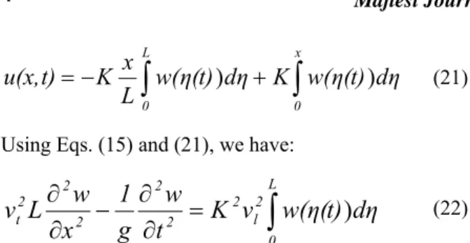
(21)

Using Eqs. (15) and (21), we have:

∫

=

∂

∂

−

∂

∂

L 0 2 l 2 2 2 2 2 2 t

K

v

w(

η

(

t)

d

η

t

w

g

1

x

w

L

v

)

(22)

Using the method of separation of variables, one will get:

)

(

)

(

)

,

(

x

t

g

x

h

t

w

=

(23) 0 ) ( ) (_{t +}T 2_{h t =} h ω ρ && ₍₂₄₎

∫

= + ′′ Lg d LT EA K x g x g 0 0 2 2 _{( ) ( )} ) (

ω

η

η

(25)

By defining a dimensionless parameter S (S=x/L) we have:

∫

= + ′′ 1 0 2 2 ) ( ) ( ) (S Ω g S λ g σ dσ g (26) in which: 0 2 2 ( ) T EA KL =

λ

₍₂₇₎

Eigenvalues of the Eq. (26), which are the natural frequencies of the suspended cable, can be calculated from Eq. (24): 2 2 1 2 2 2 0 2

*

ω

ω

π

ω

ρ

ω

=

T

=

L

_L (28)

In above equation ωL1 is the first natural frequency of an ordinary over hanged cable, furthermore in Eq. (26) following definition is also considered

2 1 2 2 2 2 2 * L L

ω

ω

π

ω

Ω

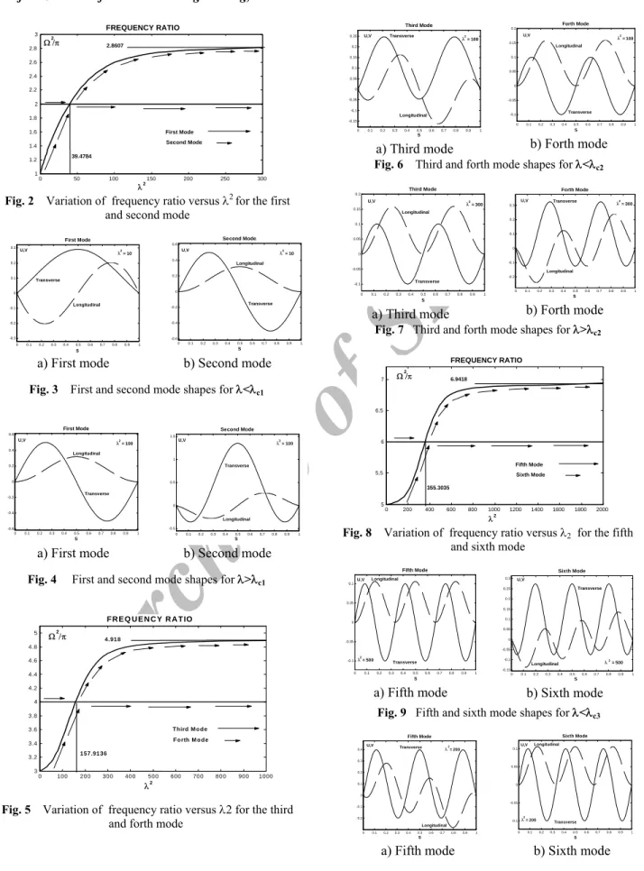
≡ = (29)

According to the previous described algorithm, natural frequencies and mode shapes of a suspended cable are calculated and plotted versus dimensionless λ.

As it is seen from Fig. 2, for different values of λ less than λc1 (in which the first crossover phenomenon is

occurred) the ratio of first natural frequency of the suspended cable to the first natural frequency of straight ordinary cable is increased and then after λc1

remains constant. Also it is seen that for values less

than the value of λc1 by increasing the value of λ, the

ratio of second natural frequency of the suspended cable to the first natural frequency of straight ordinary cable remains constant and for the values greater than

λc1 primarily it increases in a non-linear fashion and

finally approaches to the value of 2.8607.

In Fig. 3 for the values of λ less than λc1, the first

transversal mode has a symmetric shape and the second transversal mode shape is similar to the second mode shape of straight ordinary cable and for values greater than λc1, the first transversal mode shape is similar to

the second mode shape of straight ordinary cable and the second mode has a unsymmetrical shape (Fig. 4). Similar to the first and second mode shape, as it is illustrated in Fig. 5 for the values of λ less than λc2 (in

which the second crossover phenomenon is occurred) the ratio of third natural frequency of the suspended cable to the first natural frequency of straight ordinary cable is increased and then after λc1 remains constant.

Also it is seen that before λc2 with increase of the value

of λ, the ratio of forth natural frequency of the suspended cable to the first natural frequency of straight ordinary cable remains constant and for values greater than λc2 it increases and finally approaches to

the value of 4.918. In Fig. 6 for the values of λ less than λc2, third transversal mode has a symmetric shape

and forth transversal mode shape is similar to the forth mode shape of straight ordinary cable and after λc2,

third transversal mode shape is similar to the forth mode shape of straight ordinary cable and forth mode has a unsymmetrical shape (Fig. 7). From Figs. 8 to 10 it can be seen that the variation of fifth and sixth natural frequencies and mode shapes of the suspended cable is similar to that of previous modes.

Table 1 Limit values of frequency ratio and values of λ2 in

which crossover is occurred

Mode Numbers λ2c Crossover Frequency Limit Frequency Ratio 1-2 39.4784 2.8607 3-4 157.9136 4.918 5-6 355.30357 6.9418 7-8 631.6546 8.9548 9-10 986.9604 10.9631

Specific values of λ2 in which crossover phenomenon

are occurred and also the limiting values of Ω2/π are

also presented in Table 1. It is notable that all of obtained results in this paper are in a very good agreement with those given in [1] – [5].

Archive of SID

0 50 100 150 200 250 300 1 1.2 1.4 1.6 1.8 2 2.2 2.4 2.6 2.8 3 FREQUENCY RATIO First Mode Second Mode λ Ω /π 2 2 2.8607 39.4784

Fig. 2 Variation of frequency ratio versus λ2 _{for the first}

and second mode

a) First mode b) Second mode

Fig. 3 First and second mode shapes forλ<λc1

a) First mode b) Second mode

Fig. 4 First and second mode shapes forλ>λc1

0 100 200 300 400 500 600 700 800 900 1000 3 3.2 3.4 3.6 3.8 4 4.2 4.4 4.6 4.8 5 FR E Q U E N C Y R A T IO Third M o de Fo rth M o de λ Ω /π 2 2 4.918 157.9136

Fig. 5 Variation of frequency ratio versus λ2 for the third

and forth mode

a) Third mode b) Forth mode

Fig. 6 Third and forth mode shapes forλ<λc2

a) Third mode b) Forth mode

Fig. 7 Third and forth mode shapes forλ>λc2

0 200 400 600 800 1000 1200 1400 1600 1800 2000 5 5.5 6 6.5 7 FREQUENCY RATIO Fifth Mode Sixth Mode λ Ω /π 2 2 6.9418 355.3035

Fig. 8 Variation of frequency ratio versus λ2 for the fifth

and sixth mode

a) Fifth mode b) Sixth mode

Fig. 9 Fifth and sixth mode shapes forλ<λc3

a) Fifth mode b) Sixth mode

Fig. 10 Fifth and sixth mode shapes forλ>λc3

0 0.1 0.2 0.3 0.4 0.5 0.6 0.7 0.8 0.9 1 -0.3 -0.2 -0.1 0 0.1 0.2 0.3 First Mode S U,V Transverse Longitudinal λ 2 = 10 0 0.1 0.2 0.3 0.4 0.5 0.6 0.7 0.8 0.9 1 -0.6 -0.4 -0.2 0 0.2 0.4 0.6 Second Mode S U,V Transverse Longitudinal λ 2 = 10 0 0.1 0.2 0.3 0.4 0.5 0.6 0.7 0.8 0.9 1 -0.6 -0.4 -0.2 0 0.2 0.4 0.6 First Mode S U,V Transverse Longitudinal λ 2 = 100 0 0.1 0.2 0.3 0.4 0.5 0.6 0.7 0.8 0.9 1 -0.5 0 0.5 1 1.5 Second Mode S U,V Transverse Longitudinal λ 2 = 100 0 0.1 0.2 0.3 0.4 0.5 0.6 0.7 0.8 0.9 1 -0.15 -0.1 -0.05 0 0.05 0.1 0.15 0.2 0.25 Third Mode S U,V Transverse Longitudinal λ 2 = 100 0 0.1 0.2 0.3 0.4 0.5 0.6 0.7 0.8 0.9 1 -0.1 -0.05 0 0.05 0.1 0.15 0.2 Forth Mode S U,V Transverse Longitudinal λ 2 = 100 0 0.1 0.2 0.3 0.4 0.5 0.6 0.7 0.8 0.9 1 -0.1 -0.05 0 0.05 0.1 0.15 0.2 Third Mode S U,V Transverse Longitudinal λ 2 = 300 0 0.1 0.2 0.3 0.4 0.5 0.6 0.7 0.8 0.9 1 -0.2 -0.1 0 0.1 0.2 0.3 Forth Mode S U,V Transverse Longitudinal λ 2 = 300 0 0.1 0.2 0.3 0.4 0.5 0.6 0.7 0.8 0.9 1 -0.1 -0.05 0 0.05 0.1 Fifth Mode S U,V Transverse Longitudinal λ 2 = 500 0 0.1 0.2 0.3 0.4 0.5 0.6 0.7 0.8 0.9 1 -0.15 -0.1 -0.05 0 0.05 0.1 0.15 0.2 0.25 0.3 Sixth Mode S U,V Transverse Longitudinal λ 2 = 500 0 0.1 0.2 0.3 0.4 0.5 0.6 0.7 0.8 0.9 1 -0.2 -0.1 0 0.1 0.2 0.3 0.4 Fifth Mode S U,V Transverse Longitudinal λ 2 = 200 0 0.1 0.2 0.3 0.4 0.5 0.6 0.7 0.8 0.9 1 -0.1 -0.05 0 0.05 0.1 Sixth Mode S U,V Transverse Longitudinal λ 2 = 200

Archive of SID

4 NONLINEAR VIBRATION ANALYSIS OF A

MOVING CABLE WITH HARMONIC TENSION AND SPEED

Galerkin’s method is used as the solution technique. In this method, solution is approximated with the below equation: ) ( ) ( ) , ( 1 t q x t x W _n n n

∑

∞ = = Φ ₍₃₀₎

In which, Φ is the mode shape functions and q(t) is unknown functions of time to be determined. Substituting Eq. (30) into Eq. (17), for a four-term approximation one can reach

2 2 1 1 1 2 0 0 2 4 2 4 3 2 1 1 3 2 2 2 1 2 1 4 ( ) 2 (2.66 1.06 ) (2.66 1.06 ) 48.7 348.34 194.81 779.27 P V q q P V V q q V q q q q q E L q q q q ρ _ω ρ ρ − Α + = − Α − + + ⎡ − ⎤ − ⎢ ⎥ + + ⎢ ⎥ ⎣ ⎦ && & & & (31) 2 2 2 2 2 2 0 0 1 3 1 3 2 2 1 2 3 2 3 2 2 2 4 ( ) 2 (2.66 4.8 ) (2.66 4.89 ) 194.8 1753.36 779.27 3117 P V q q P V V q q V q q q q q E L q q q ρ _ω ρ ρ − Α + = − Α − − − − ⎡ + ⎤ − ⎢ ⎥ + + ⎢ ⎥ ⎣ ⎦ && & & & (32) 2 3 3 3 3 2 0 4 2 4 2 2 2 3 1 3 2 3 2 3 2 3 4 ( ) 2 (6.85 4.8 ) (6.85 4.8 ) 438.34 3945 1753.36 7013.45 P V q q P V V q q V q q q q q E L q q q q ρ _ω ρ ρ − Α + = − Α − + − ⎡ + ⎤ − ⎢ ⎥ + + ⎢ ⎥ ⎣ ⎦ && & & & (33) 2 2 4 4 4 2 0 0 3 1 3 1 2 2 4 1 4 3 2 2 3 4 2 4 ( ) 2 (6.85 1.06 ) (6.85 1.06 ) 779.27 7013.45 3117.09 12468.36 P V q q P V V q q V q q q q q q E L q q q ρ _ω ρ ρ − Α + = − Α − + − + ⎡ + +⎤ − ⎢ ⎥ + ⎢ ⎥ ⎣ ⎦ && & & & (34) 5 VALIDATION OF SIMULATION

A special case of a moving viscoelastic cable with constant tension and speed [12] in the literature is considered in this section. For such a special case differential equations of motion can be derived as [12]

) , ( 1 ) ( ) ( 2 ₂ 2 2 2 2 2 t x f x w x x w P V x t w V t w Α σ Α ρ ρ ρ + ∂ ∂ ∂ ∂ = ∂ ∂ − + ∂ ∂ ∂ + ∂ ∂ (35)

For such a viscoelastic cable with constant velocity and tension, numerical simulations have been carried out and the obtained results are compared with [12] in Fig. 11. As it is illustrated a very good correlation is seen between the results.

Fig. 11 Comparison between the results from the present

work (Right) and [12] (Left)

6 NUMERICAL RESULTS

Using the prescribed method of solution provided for differential equations of motion a computer program has been written employing MATLAB (R2006b) software and a comprehensive parametric study is carried out. 4th order Runge-Kutta method with time increment of 0.01 is employed in numerical integrations.

Archive of SID

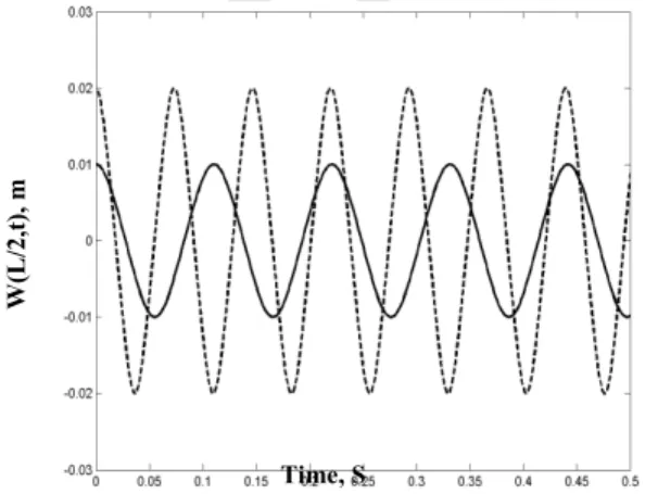
For a real case with mechanical properties listed in

Table 2, different approximations for the response of the midpoint of the cable are illustrated in Figs. 12 to 14. Effects of the initial conditions on the frequency of the free vibrations of the moving cable are illustrated in Fig. 11. As it is seen the dynamic system has hardening behavior and the period of its vibration decreases with increasing of the magnitude of initial condition.

Table 2 Mechanical properties of the simulated belt

Symbol Value Unit

ρ 7.68X103 _kg/m3 A 4 X10-5 _m2 L 1.0 m E 3X109 _N/m2 P0 76.22 N V0 10 m/s ε1=ε2 0.1

Effects of the harmonic tension on reduction of the vibration amplitude are illustrated in Fig. 13. As it is seen the harmonic tension force acts as the control force and reduces the amplitude of vibration even up to 10%. This means that if the moving cable is excited with the harmonic variable tension with the same frequency and phase of the natural vibration the vibration amplitude will decrease noticeably. That result is quite matched with physical experience when someone applies a harmonic tension on a vibrating rope with the same frequency and phase of its vibration to suppress the oscillations. Effects of the amplitude of harmonic tension on reduction of the vibration amplitude are illustrated in Fig. 14. As it is seen, amplitude of vibration reduces by increasing of the amplitude of the variable tension.

Fig. 12 Effect of the initial condition on the period of free

vibration

Fig. 13 Effect of the harmonic tension on reduction of the

vibration amplitude

Fig. 14 Effect of the amplitude of harmonic tension on

reduction of the vibration amplitude

Fig. 15 Effect of the frequency of harmonic tension on

reduction of amplitude Time, S W(L/2,t) , m W(L/2,t) , m Time, S Ω1=1.0*ω1=42.83 Rad/s Ω2=0 V*=4 m/s P*=0 N Ω1=1.0*ω1=42.83 Rad/s Ω2=1.0*ω1=42.83 Rad/s V*=4 m/s P*=40 N P*=20 N P*=30 N P*=40 N ( Ω1=1.0*ω1=42.83 Rad/s Ω2=1.0*ω1=42.83 Rad/s V*=4 m/s ) Time, S W(L/2 ,t) , m ( Ω1=1.0*ω1=42.83 Rad/s V*=4 m/s P*=40 N ) Time, S W(L/2,t) , m Ω2= 0.5*ω1=21.42 Rad/s Ω2= 1.0*ω1=42.83 Rad/s Ω2= 1.5*ω1=64.24 Rad/s

Archive of SID

Effects of the frequency of harmonic tension on

reduction of the vibration amplitude are illustrated in Fig. 15. As it is seen, the variable tension acts as a controller force to reduce the vibration of the cable. It is seen that if the frequency of the variable tension is exactly equal to the first natural frequency of the cable, it has its highest performance in reducing the vibration level of the cable.

7 CONCLUSION

Coupled nonlinear vibrations of a suspended cable with time dependent tension and velocity were studied in this paper. For a stationary sagged cable a modal analysis was initially carried out in order to identify the dynamic system. A crossover phenomenon was achieved in which two consecutive natural frequencies become the same. Natural frequencies and mode shapes are plotted versus a dimensionless parameter λ, known as static sag character. In case of moving cable, the tension force and the rotary speed of the pullies were assumed to be harmonic functions. Galerkin mode summation approach was employed to discretize the nonlinear equations of motions. Numerical simulations were carried out in the time domain. A frequency analysis was then carried out and effects of the frequency of tension force and rotary speed on the belt dynamic responses are studied. Validity of the simulation was verified for a special case in the literature i.e. a moving cable with constant tension and sinusoidal speed. It was proved that the nonlinear dynamic system of a moving cable with variable tension and speed acts a hardening system and the period of its vibration decreases with increasing of the magnitude of initial condition. It was also found that fourth order Galerkin approximation is an acceptable solution with very good convergence. A comprehensive parametric study was carried out and effects of different parameters like the moving speed and tension force on the response were studied. It was also found that the harmonic tension can act as a suppression system and reduces the amplitude of vibration.

Nonlinear vibration of a moving belt with time dependent tension and velocity was studied in this paper. Tension force and the moving speed were assumed to be harmonic. Dynamic responses of the system were calculated using Galerkin’s method. A frequency analysis was carried out and effects of different parameters like the moving speed and tension force on the responses were studied. it was proved that increasing the tension increases the critical speed of the

moving cable. It was also found that the harmonic tension can act as a controller and reduces the amplitude of vibration up to 25 times. Optimal frequency of the variable tension was found to be exactly the first natural frequency of the systems and also it was proved that increasing the amplitude of the variable tension can considerably reduce the level of vibration. It was found that the behavior of the systems is harmonic when the excitation frequency is much or less than the natural frequency. Exactly at the natural frequency the system has beating behavior and the frequency of beating increases with increase of the amplitude of variation of the moving speed and also the variable tension.

REFERENCES

[1] Irvin, H. M., and Caughey, T. K., “The Linear Theory of

Free Vibration of Suspended Cables,” Proc. Royal. Soc. London A341, 1974, pp. 299-315.

[2] Irvin, H. M., “Cable Structures,” MIT Press, 1981.

[3] Rega, G. and et al, “Parametric Analysis of Large

Amplitude Free Vibrations of Suspended Cable,” Int. J. Solids and Structures, Vol. 20, No. 2, 1984, pp. 95-105.

[4] Perkins, N. C., and Mote, C. D., “Three-Dimensional

Vibration of Traveling Elastic Cables,” J. Sound and Vibration, Vol. 114, No. 2, 1987, pp. 325-340.

[5] Scholar, C., and Perkins, N. C., “Low Order Vibration

Models for Tracked Vehicles,” Proc. ASME Design Engineering. Nevada DETC99/VIB-8201, 1999.

[6] Assanis, D. N., and et al, “Modeling and Simulation of

an M1 Abrams Tank with Advanced Track Dynamics and Integrated Virtual Diesel Engine,” Automotive Research Center Report, The University of Michigan Ann Arbor, MI 48109–2125, 1999.

[7] Reddy, J. N., “Applied Functional Analysis and

Variational Methods in Engineering,” Mc Graw-Hill, 1986.

[8] Sofi, A. and Muscolino, G., “Dynamic Analysis of

Suspended Cables Carrying Moving Oscillators”, International Journal of Solids and Structures, Vol. 44, 2007, pp. 6725-6743.

[9] Chen L-Q., Zhang, W., and Zu J.W., “Nonlinear

Dynamics for Transverse Motion of Axially Moving Strings, Chaos,” Solutions and Fractals, Vol. 40, 2009, pp. 78–90.

[10]Chen, L-Q., Chen, H. and Lim, C.W., “Asymptotic

Analysis of Axially Accelerating Viscoelastic Strings,” International Journal of Engineering Science, Vol. 46, 2008, 976–985.

[11]L-Q. Chen, “Analysis and Control of Transverse

Vibrations of Axially Moving Strings”, Vol. 58, 2005, pp. 91-115.

[12]Wei-jia, Zh., Li-qun, Ch., and Zu J. W., “A Finite

Difference Method for Simulating Transverse Vibrations of an Axially Moving Viscoelastic String,” Applied Mathematics and Mechanics (English Edition), Vol. 27, No. 1, 2006, pp. 23-28.